Tutorial 2.2
QBO: Description of experimental apparatus
Alan Plumb and Angus McEwan's experiment (Plumb & McEwan 1978) was intended to reproduce the ‘spirit’ of Richard Lindzen and James Holton's QBO mechanism (Lindzen & Holton 1972), both to illustrate it and to verify that it would actually work in a real fluid!
Such experimental verification is an important element of the scientific process in making sure that a simple and highly idealised theory can actually achieve what is claimed without other complications or instabilities overwhelming the main result. In this case, it turned out to be easier to carry out the experiment in a non-rotating apparatus, using directly forced internal gravity waves to play the part of the Kelvin and mixed Rossby–gravity waves of Lindzen & Holton 1968. The latter only relied on having upward propagating waves which included those with components of their phase velocity in either zonal (azimuthal) direction – so ought to work in principle with almost any kind of waves. In fact the details of the theory using non-rotating internal gravity waves had also been worked out previously in Plumb 1977.
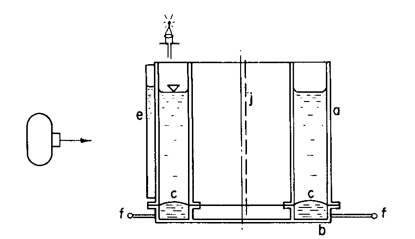
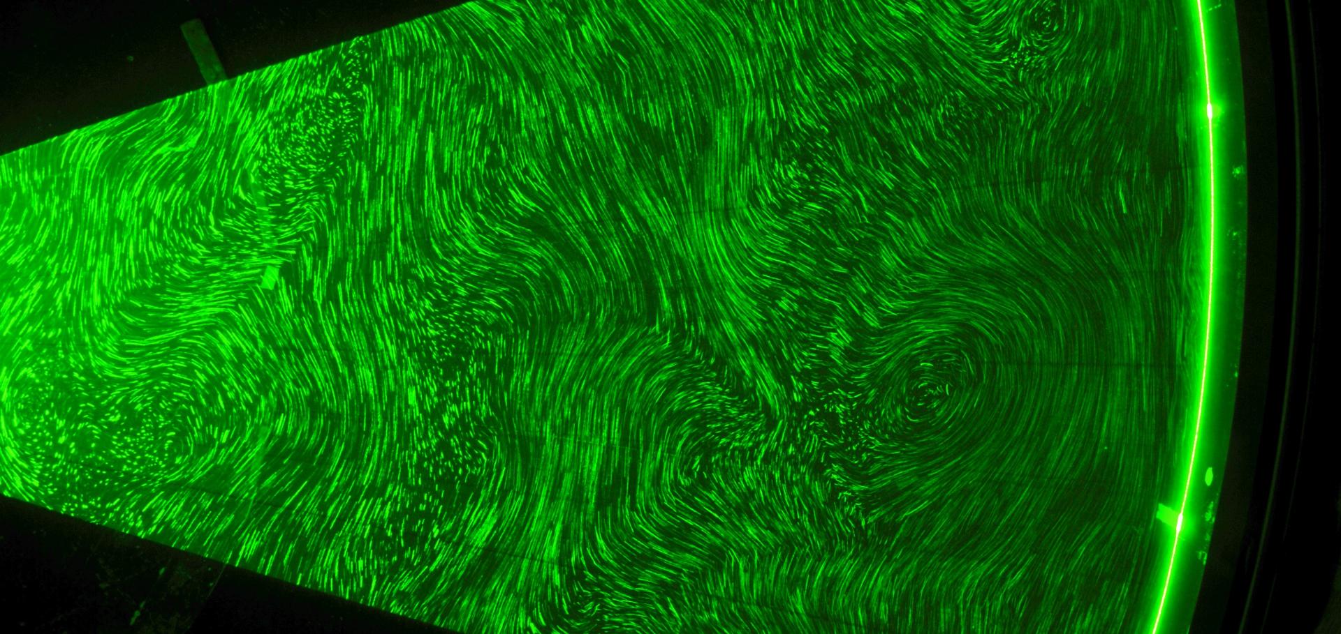
The experiment was performed in an annular tank (in order to permit azimuthal flow – see Figs. 2.2a and 2.2b, taken from Plumb & McEwan 1978). This tank was filled with linearly stratified salt water, allowing for the propagation of internal gravity waves. A forced standing wave – equivalent to an ‘easterly’ plus a ‘westerly’ wave – was launched from the lower boundary by periodically oscillating a segmented membrane on the bottom (see above). The standing wave would then propagate upward through the fluid, where it was damped by viscosity.
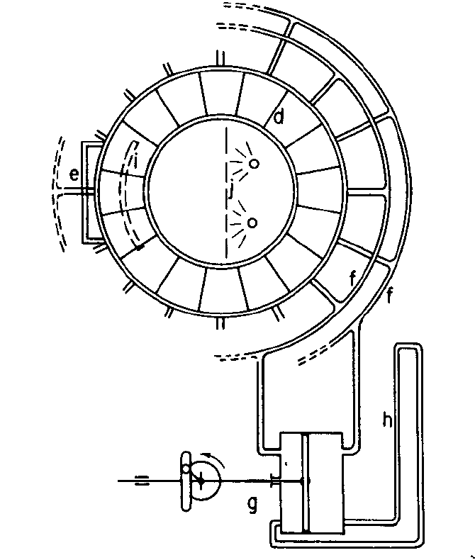
The rubber membrane was sealed to 16 partitions in the lower annulus. Alternate segments were pumped up and down by a piston (labelled g above). Thus the membrane performed a standing oscillation (of wavenumber \(m=8\)), whose amplitude and frequency could be controlled.
Experimental parameters
Annulus dimensions:
- Inner radius: \(a=0.183\text{ m}\)
- Outer radius: \(b=0.300\text{ m}\)
- Height: \(d=0.500\text{ m}\)
- Fluid kinematic viscosity: \(1.0\times10^{-6}\text{ m}^2\text{ s}^{-1}\)
- Forcing wavenumber: \(m=8\)
- Fluid depth: \(D\sim0.4\text{ m}\)
- Buoyancy frequency: \(N\sim1.5\text{ s}^{-1}\)
Forced standing wave on lower boundary:
- Frequency: \(w=0.4\text{ s}^{-1}\)
- Amplitude: \(e=10\text{ mm}\)
In each experiment, the fluid was virtually at rest when forcing was commenced. The filmed sequences were taken after two to three hours, by which time the motion had settled down into a regular state.