Tutorial 0
Dynamical features of fluids in rotation
As with other mechanical systems that involve rapid rotation, systems of rotating fluids have a number of distinctive dynamical properties that make them behave rather differently to fluids in inertial or stationary reference frames.
Rigid bodies in rotation, such as gyroscopes, acquire extra inertia that resists changes to the direction of the rotation axis, and leads to responses to applied forces and torques that act perpendicularly to them. For some demonstrations of this effect, see the following videos:
(click links to view videos)
mittechtv, ‘MIT Physics Demo -- Bicycle Wheel Gyroscope’
ScienceOnline, ‘Gyroscope’
Fluids also exhibit gyroscopic effects that give the fluid a kind of ‘stiffness’ in the direction of the rotation axis. This can result in homogeneous, unstratified fluids behaving as if they were two-dimensional, with a kind of coherence along the direction of the rotation axis. Physically, rotating reference frames are accelerating and therefore not like inertial frames. This leads to the appearance of apparent accelerations (‘fictitious forces’) acting on motion relative to a rotating reference frame in the form of centrifugal and Coriolis accelerations.
The Coriolis ‘force’ (per unit mass), in particular, takes the form \(2\mathbf{\Omega}\times\mathbf{u}\), and therefore acts perpendicularly to both the rotation axis (which is in the same direction as the angular velocity \(\mathbf{\Omega}\)) and the local velocity \(\mathbf{u}\). For a strong enough rotation speed \(\mathbf{\Omega}\), this can become the dominant force in the flow so that in a steady state the equation of motion (i.e. Newton’s second law) reduces to a balance between Coriolis and pressure-gradient forces: \[2\mathbf{\Omega}\times\mathbf{u} = -\frac{1}{\rho} \nabla p\] This effect is known as geostrophic balance. This means that fluids tend to flow parallel to contours of pressure \(p\) (isobars) – much as seen on weather maps – and not down the pressure gradient as in non-rotating flows.
This situation is found when other forces (such as friction or inertial accelerations) are relatively small. This occurs when dimensionless numbers such as the Ekman number \[\mathrm{Ek} \approx \frac{\lvert v \nabla^2 \mathbf{u}\rvert}{\lvert 2\mathbf{\Omega}\times\mathbf{u}\rvert} \approx \frac{v}{2\Omega L^2}\] and the Rossby number \[\mathrm{Ro} \approx \frac{\lvert \mathbf{u} \cdot \mathbf{\nabla u}\rvert}{\lvert 2\mathbf{\Omega}\times\mathbf{u}\rvert} \approx \frac{U}{2\Omega L}\] are both \(\ll1\).
If we take the curl of the first equation (for geostrophic balance), we can use the fact that, for a homogeneous incompressible fluid, \(\mathbf{\nabla}\cdot\mathbf{u}=0\) and \(\rho\) is constant, to reduce the equation to the form: \[(2\mathbf{\Omega}\cdot\mathbf{\nabla})\mathbf{u}=0\]
This basically means that steady or slowly evolving flows do not vary along the direction of the rotation axis, and essentially behave like a two-dimensional flow. This is often referred to as the Taylor–Proudman theorem, after the theoretical work of Joseph Proudman (1916) and the first experimental demonstration of the effect by Geoffrey Ingram Taylor (1923). This is related to the gyroscopic stability of a rotating rigid body, since it expresses the resistance of an initially coherent column of fluid parallel to the rotation axis (known as a Taylor column) from tilting over or changing direction.
Here we show a demonstration of such a Taylor column, originally set up by Clive Titman at Newcastle University in the 1970s (for more details, see chapter 15 of Physical Fluid Dynamics – Tritton 1977 or 1988). The setup is shown in the figure below. A shallow truncated cylindrical obstacle is placed in a rotating cylindrical tank of water. A slow, steady azimuthal flow is driven by slowly pumping water in through the porous side wall and out through a sink at the centre of the tank. The flow is mainly azimuthal because of the rapid rotation, so that Coriolis accelerations balance those due to the imposed radial pressure gradient.
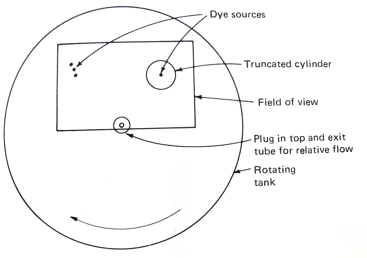
The flow is visualised by injecting dye into it at two separate locations:
- (a) at a set of three point sources located upstream of the obstacle and well above its top
- (b) on the top of the truncated cylinder itself
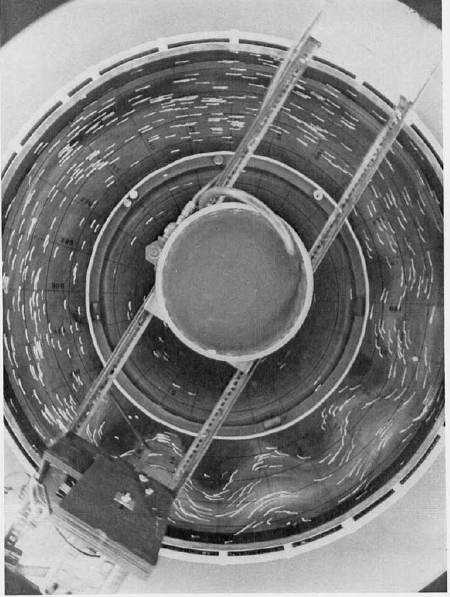
The movies below show how the azimuthal motion flows around the truncated cylinder, even at levels above the top of the obstacle. Within the Taylor column above the cylinder the flow is very sluggish and disconnected from the azimuthal flow outside.
https://youtu.be/XQoX5vfzzgY https://youtu.be/h4lOHXjtSdQ
For other demonstrations of the Taylor–Proudman theorem, see also:
ucla spinlab, ‘Record Player Fluid Dynamics: A Taylor Column Experiment’
Allison Wing, ‘Taylor Columns’
ESSC CUHK, ‘06 Taylor Columns’
Adding time dependence to the first equation allows for the possibility of wave motion in the form of inertial waves, which are highly dispersive and can propagate as long as the frequency \(\omega\ll2\Omega\). When \(\mathrm{Ek}\) and \(\mathrm{Ro}\) are both \(\ll1\), the vorticity equation reduces to the form \[\frac{\partial \zeta}{\partial t}(+\mathbf{u}\cdot\mathbf{\nabla}\zeta) = 2\Omega\frac{\partial w}{\partial z}\] where \(\zeta\) is the component of vorticity parallel to the rotation axis (the \(z\)-direction) and \(w\) is the axial velocity component. Integrating or averaging this equation along the z-direction between two rigid boundaries – i.e. \(\bar{[\,\cdot\,]}\frac{1}{h}\int\,[\,\cdot\,]\,\mathrm{d}z\), where \(h\) is the local vertical distance between the two boundaries – leads to a conservation equation for the absolute vorticity \(\bar{\xi}\equiv\bar{\zeta}+2\Omega\), of the form \[\frac{\partial}{\partial t}(+\mathbf{u}\cdot\mathbf{\nabla})\frac{\bar{\xi}}{h} = 0\] using the fact that, near each boundary, \(w=\mathbf{u}\cdot\mathbf{\nabla}h\). This means that the quantity \(q \equiv \frac{\bar{\xi}}{h}\) (known as a potential vorticity) is conserved following the (horizontal) flow.
If the boundaries slope such that \(h\) varies with the radius \(r\) so that \[\frac{2\Omega}{h}\frac{\partial h}{\partial r} = \beta\]then the vorticity equation supports a class of travelling inertial-type waves known as Rossby waves. These waves are highly dispersive and anisotropic, with a phase propagation that only goes in one direction – for more details, see e.g. Tritton 1977 or 1988, or Vallis 2017.
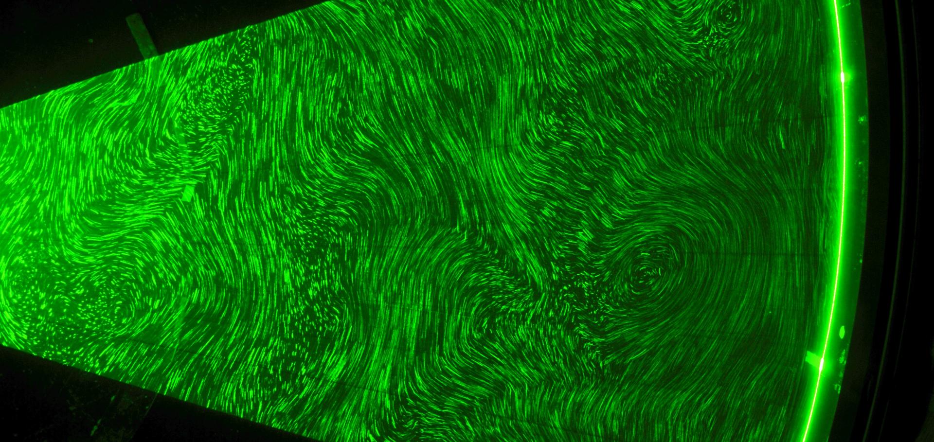
The figure below illustrates a demonstration of Rossby waves in the laboratory by Alan Faller, produced by an azimuthal flow past a bump (for more details, see Tritton 1977 or 1988 and Platzman 1968).
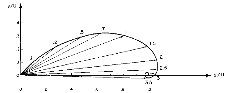
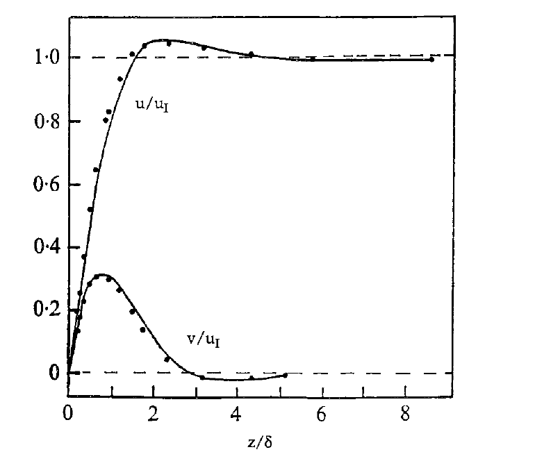
Close to horizontal or sloping rigid or free boundaries, the geostrophic flow cannot usually satisfy the usual non-slip or free-slip impermeable boundary conditions. This typically leads to the formation of a boundary layer where the viscous acceleration becomes comparable to Coriolis accelerations. This is known as an Ekman layer, named after the Swedish oceanographer Vagn Ekman (1874–1954), who discovered it through its effect on the motion of icebergs. In an Ekman layer, Coriolis accelerations deflect the flow in the boundary layer to form a spiral variation of the flow direction with \(z\). This has been nicely demonstrated in the laboratory, and examples can be seen here. The theory can be found at Tritton 1977 or 1988 and Vallis 2017. A figure illustrating the structure of an Ekman layer is shown below.
Finally, the addition of density stratification in the presence of a gravitational field \(\mathrm{g}\) modifies the Taylor–Proudman theorem to account for density gradients, taking the form: \[(2\mathbf{\Omega}\cdot\mathbf{\nabla})\mathbf{u} \approx \frac{\mathbf{g}\times\mathbf{\nabla}\rho}{\rho}\]
This shows that the vertical variation of the geostrophic flow \(\mathbf{u}\) depends on \(\mathbf{\Omega}\), \(\mathbf{g}\), and the horizontal density gradient (known as the thermal wind shear in meteorology. Together with a stable vertical density gradient, this relation links the slope of density surfaces (isopycnals) with the vertical shear of the horizontal flow. This will be important in understanding baroclinic instability and sloping convection in Tutorials 1 to 3.
More detailed discussions of these topics and the underlying theory can be found in the references below, including Raymond Hide’s 1977 Presidential Address to the Royal Meteorological Society (Hide 1977).