Tutorial 3
Circulation regimes in a planetary atmosphere
The main features of the circulation of the Earth’s atmosphere are familiar to many people, including the strong eastward (westerly) jet stream at high altitudes around the latitudes of 40° to 60° in each hemisphere, prevailing westerly winds at low levels in mid-latitudes and easterly trade winds in the tropics, and dynamically active cyclonic and anticyclonic weather systems in storm tracks associated with the mid-latitude jet streams.
But is this organisation of the circulation unique to Earth, or would it look differently on other planets of different sizes and which rotate at different speeds? How different would the Earth’s climate and circulation look if it rotated more quickly or more slowly than it does today?
One way to explore these questions systematically is to use a numerical simulation model of the atmosphere, similar to those used to forecast the weather or simulate the climate on Earth, but changing some of the parameters such as the planetary radius or rotation speed. This approach has been used since the late 1970s to investigate:
- how the Earth’s climate might have changed since life first appeared more than two billion years ago (when a day on Earth was significantly shorter than 24 hours)
- what the atmospheric circulation might look like on Earth-like planets orbiting other stars
Here we explore how the circulation changes with different rotation speeds, using simulations obtained in a simplified model, based on those used for studies of the Earth.
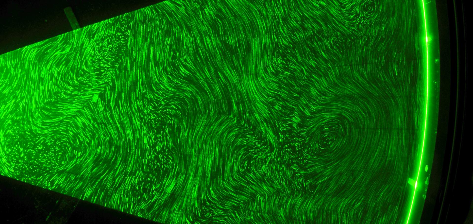
We also compare and contrast the changes in circulation regime with those found in rotating annulus experiments as parameters such as the rotation speed are varied (see Tutorial 1.1 for further details).
The model we use is based on the simplified global climate model called PUMA (Portable University Model of the Atmosphere), developed by the Meteorological Institute at the University of Hamburg in Germany. This model solves the equations of fluid dynamics, energy and mass conservation in a shallow atmosphere on a spherical planet of radius \(a\) and angular speed of rotation \(\Omega\). Heating and cooling are imposed by gently forcing the temperature in the atmosphere to tend towards a pattern in latitude and height similar to that found on Earth, as shown below:
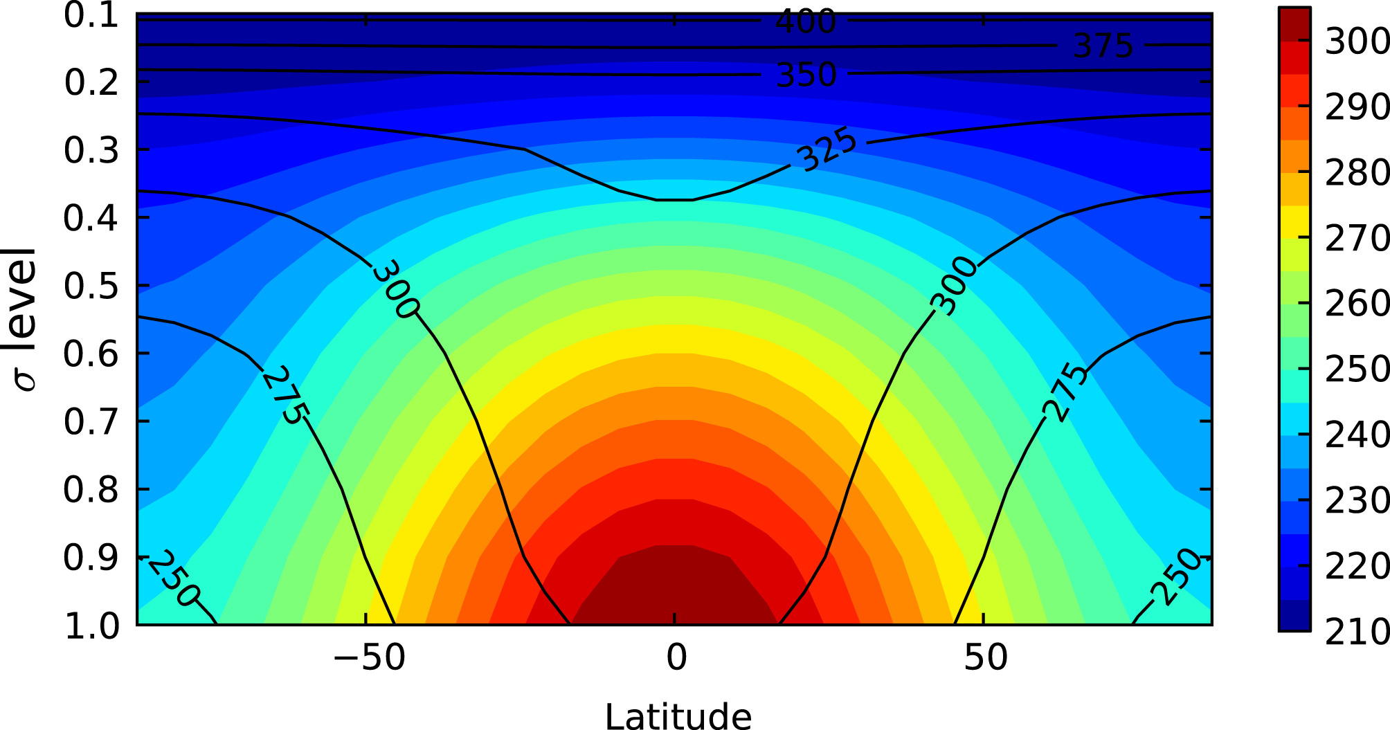
Everything else is kept very simple, including a simple representation of surface friction to close the energy budget. We then choose a rotation speed for the planet and run the model for a long time until the circulation settles down to a statistically steady state. This is then repeated for different rotation speeds, from \(\Omega=\frac{1}{16}\Omega_E\) (384 hours per day) to \(\Omega=8\Omega_E\) (3 hours per day) – \(\Omega_E\) is the Earth’s rotation rate, with one day equalling 24 hours. By analogy with the rotating annulus laboratory experiments (Tutorial 1), we can define dimensionless parameters as coordinates on a regime diagram or circulation map, with the most important being:
- a thermal Rossby number: \[\mathrm{Ro}_T = \frac{R \Delta T_h}{\Omega^2 a^2}\]
- a frictional Taylor number: \[\mathrm{Ta}_f = 4(\Omega\tau_f)^4\]
where \(R\) is the specific gas constant, \(\Delta T_h\) is the equator–pole temperature difference, and \(\tau_f\) is a frictional timescale associated with spinning down.
Regime diagram
The following regime diagram shows where different circulation regimes occur with respect to different values of \(\mathrm{Ro}_T\) and \(\mathrm{Ta}_f\):
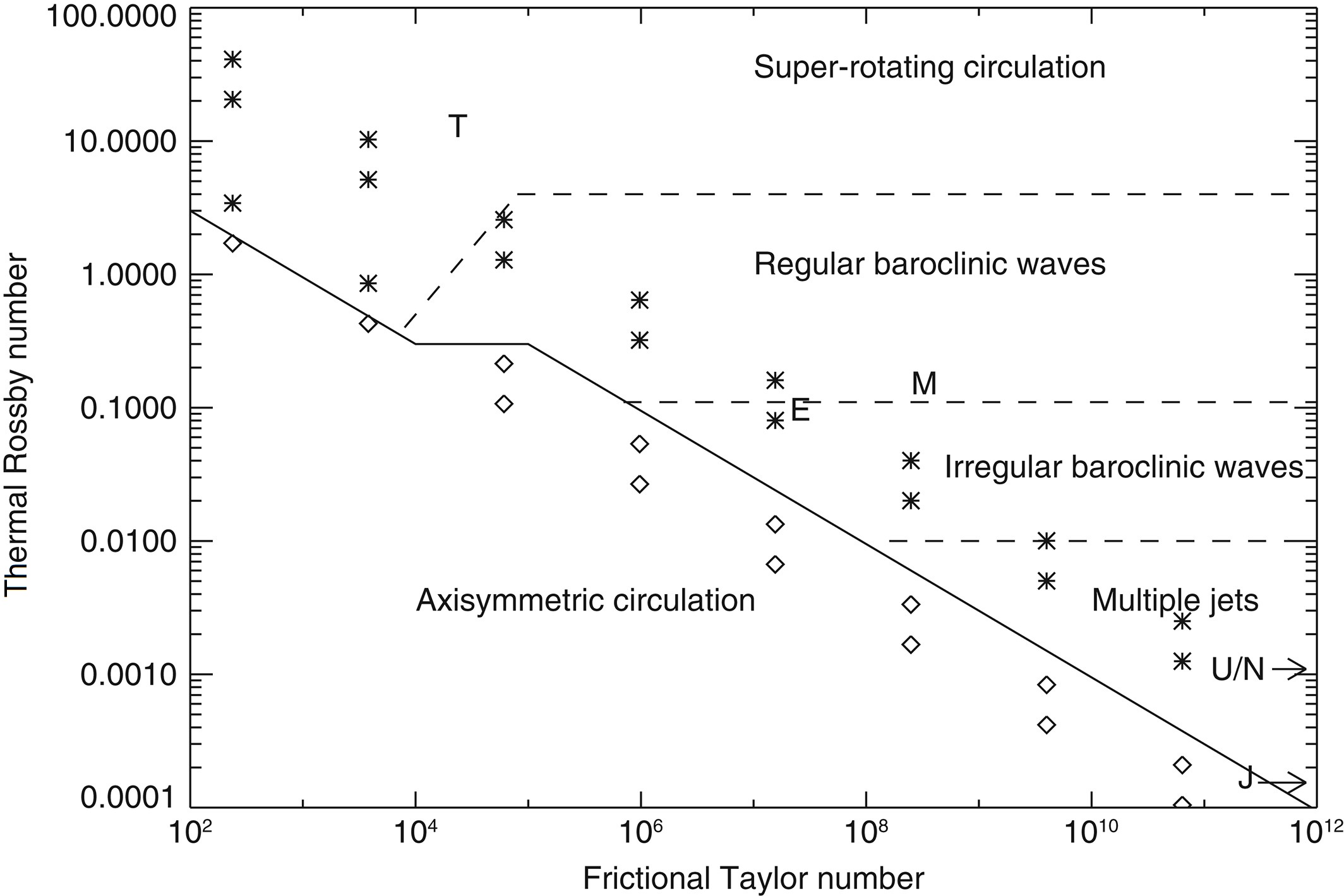
Stars refer to experiments in which wavy flows are discovered, whereas open diamonds indicate experiments in which axisymmetric flows were found.
The approximate location in parameter space of some Solar System bodies (Earth, Mars, Titan, Jupiter, Saturn, Uranus, and Neptune) are labeled by their initial letters.
The solid line delineates the boundary between axisymmetric circulations and circulations with wavy/turbulent flows. The dashed lines indicate the boundaries between different circulation regimes within the wavy/turbulent region.
The following video clips provide visualisations of flows on the regime diagram above, showing animations of zonal wind \(u\) at \(\text{200 mb}\) on the left, and atmospheric temperature \(T\) at \(\text{500 mb}\) on the right. These videos are best viewed at a larger size or full-screen – click on the video title to view it in the standard YouTube interface. For optimal effect, right-click on the video to enable looping.
(N.B.: \(\Omega^* \equiv \frac{\Omega}{\Omega_E}\))
\(\Omega^*=\frac{1}{16}\) (384 hours per day)
https://youtu.be/qVJ_vOz-C50 https://youtu.be/cdS7AsPoyfU
\(\Omega^*=\frac{1}{8}\) (192 hours per day)
https://youtu.be/sg8nkZ0tBd4 https://youtu.be/wKiZylBkzAQ
\(\Omega^*=\frac{1}{4}\) (96 hours per day)
https://youtu.be/V08Z7RJQhww https://youtu.be/Zu0fdYGkEVw
\(\Omega^*=\frac{1}{2}\) (48 hours per day)
https://youtu.be/6FzFzdYJels https://youtu.be/f1avONiJC4c
\(\Omega^*=1\) (24 hours per day)
https://youtu.be/mfVUOakL37U https://youtu.be/uiG3FI_YgwM
\(\Omega^*=2\) (12 hours per day)
https://youtu.be/N_nvZuCXkc0 https://youtu.be/3V79IfGEnbY
\(\Omega^*=4\) (6 hours per day)
https://youtu.be/OulbJxacdBs https://youtu.be/rw7l8WJXqOM
\(\Omega^*=8\) (3 hours per day)
https://youtu.be/9TzDBkJP2v8 https://youtu.be/UY0XjYSE8DY
Note similarities with the regime diagrams shown in Tutorials 1.1 and 1.5. This shows how laboratory experiments are able to provide insights that are relevant to understanding atmospheric circulation regimes.
Trends with \(\Omega\) are also evident in the patterns of wind and temperature in the zonally averaged flow:
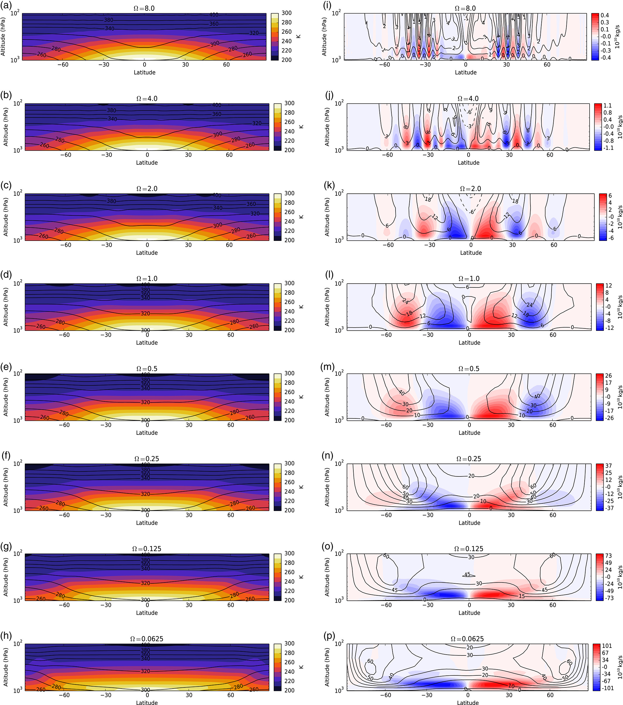
(a)–(h) temperature (absolute \(T\) and potential \(\theta\))
(i)–(p) zonal wind and meridional streamfunction
for \(\Omega^*\) equal to (a, i) \(8\); (b, j) \(4\); (c, k) \(2\); (d, l) \(1\); (e, m) \(\frac{1}{2}\); (f, n) \(\frac{1}{4}\); (g, o) \(\frac{1}{8}\); and (h, p) \(\frac{1}{16}\).
Shading indicates absolute temperature in (a)–(h) and meridional streamfunction in (i)–(p), while contours indicate potential temperature in (a)–(h) and zonal velocity in (i)–(p).
Temperature contrasts with latitude become much weaker on slowly rotating planets compared to fast rotators. At slower rotation rates, the mid-latitude jet stream also moves towards the poles, but at fast rotation speeds instead moves towards the Equator and breaks up into multiple jets. These trends seem to be reflected in other Solar System planets, comparing slow rotators (such as Venus or Titan) with Earth-like rotators (such as Mars) and fast rotators (such as Jupiter or Saturn).
Heat transport
The efficiency by which heat is transported from the tropics to the polar regions also varies strongly with the planetary rotation speed. The figure below shows how the maximum poleward transport of heat energy varies with \(\Omega\) and \(\mathrm{Ro}_T\):
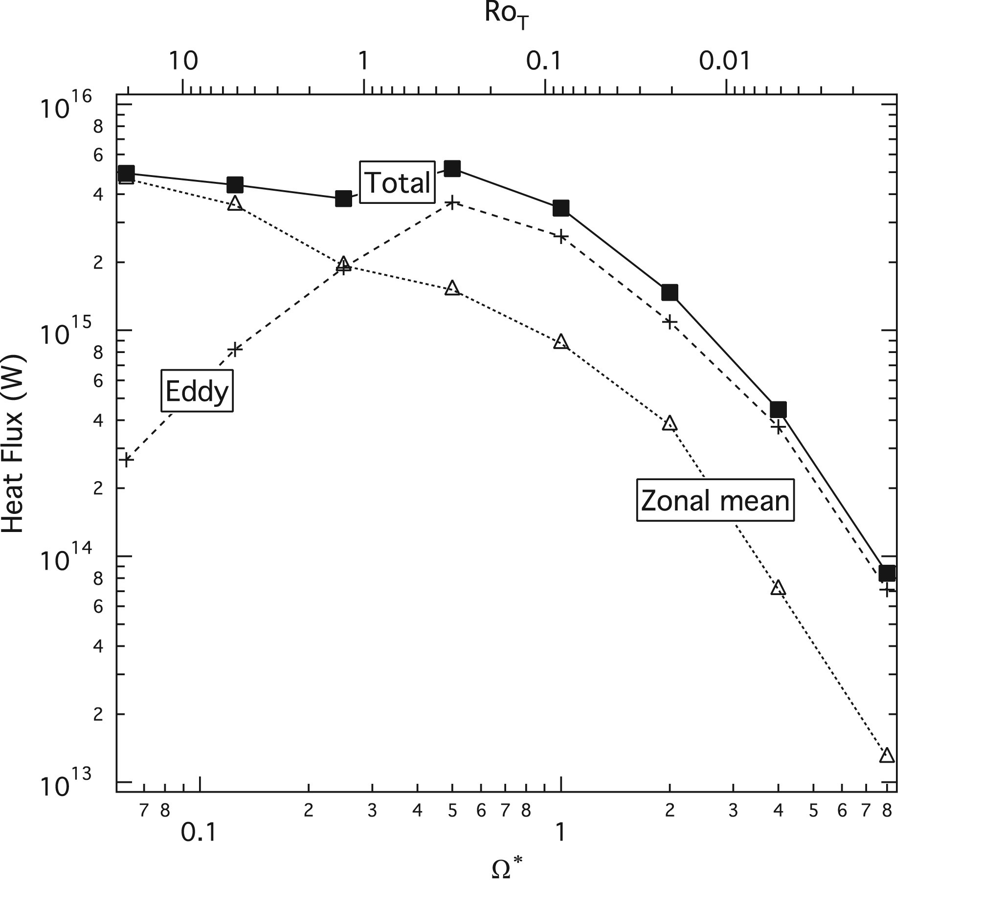
Squares: total poleward transport
Triangles: zonal mean transport (\(\int_0^\infty \rho c_\text{p} \overline{v T'} \frac{\mathrm{d}p}{g}\))
Crosses: eddy transport (\(\int_0^\infty \rho c_\text{p} \overline{v^* T^*} \frac{\mathrm{d}p}{g}\))
The total transport is shown also broken down into contributions from the zonally symmetric meridional overturning (zonal mean) and baroclinic eddies. Note that the total heat transport is almost independent of \(\Omega\) (at around \(5\times10^{15}\text{ W}\)) for rotation speeds less than the Earth’s rotation rate, but decreases sharply at faster speeds. This is because the eddy and zonal mean contributions roughly compensate each other for \(\Omega < \text{1 day}^{-1}\), but both decrease with \(\Omega\) for \(\Omega > \text{1 day}^{-1}\).