Tutorial 1.2
Vertical structure of baroclinic annulus waves
Baroclinic instability, as its name implies, is a three-dimensional process that entails the transport of heat both upwards and horizontally, ‘down’ the zonal mean horizontal temperature gradient. This means that the baroclinic waves resulting from this instability must have a quite complicated vertical and horizontal structure.
- The pressure \(p\) varies approximately sinusoidally in azimuth/longitude, so that the pressure gradient force can support radial geostrophic flow to transport heat horizontally.
- The temperature \(T\) is related to \(\frac{\mathrm{d}p}{\mathrm{d}z}\) (via hydrostatic balance) so, in order to result in heat transport, the pressure \(p\) must also vary with the height \(z\). In practice, this usually results in a ‘westward’ phase tilt with the height of the pressure field. \(T\) must also then vary approximately sinusoidally in azimuth/longitude, and in the vertical with a phase tilt that is consistent with \(p\).
- The vertical velocity \(w\) will also vary approximately sinusoidally within the wave, and will develop a pattern that leads to a positive correlation between \(w\) and \(T\). This is necessary to ensure upward heat transport - necessary to release buoyant potential energy. However, \(w\) must also be consistent with the geostrophically balanced horizontal flow, for instance through the quasi-geostrophic omega equation.
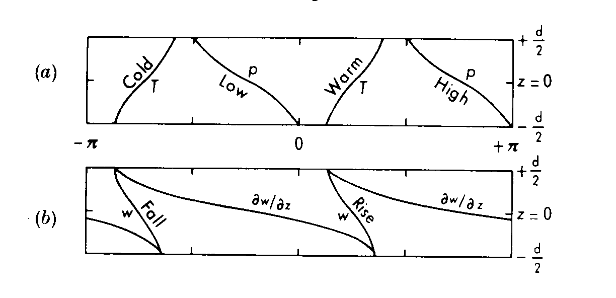
This kind of three-dimensional multivariate pattern can be seen, for example, in the structure of a growing Eady wave. The figure below shows a schematic illustration of the phase lines in the zonal and vertical directions at fixed latitude for the most rapidly growing unstable Eady mode (Eady 1949). This clearly shows the westward phase tilt with height of \(p\) and a generally eastward phase tilt for \(T\). The phase lines for \(w\) are consistent with an upward vertical velocity occurring mostly where the temperature part of the wave is relatively warm, and vice versa for the downward branch of the wave.
This kind of structure is evident in real baroclinic waves, such as in the rotating annulus experiments in the laboratory. The figure below shows the structure of the pressure, temperature and vertical velocity fields as contours in azimuth and height at mid-channel in a numerical simulation of a fully developed flow with \(m=3\) in a thermally driven rotating annulus. In this case the detailed structure of the wave in \(p\), \(T\) and \(w\) is somewhat different to the Eady wave, but still shows similar characteristics.
Remarks:
- The pressure \(p\) still exhibits a ‘westward’ phase tilt with height \(z\), though with a somewhat different amplitude structure from the Eady wave.
- The temperature \(T\) follows \(\frac{\mathrm{d}p}{\mathrm{d}z}\) fairly closely, with a generally eastward phase tilt with height \(z\), though with more complicated structure near the Ekman boundary layers.
- The vertical velocity \(w\) looks rather different from the Eady wave, though still shows the required correlation with \(T\) to achieve upward heat transport.
- It is surprising how closely these simulations of fully developed baroclinic waves resemble the structure of growing Eady waves, given that the latter are solutions to a highly idealised, linear model of baroclinic instability.
Laboratory visualisations of baroclinic flows
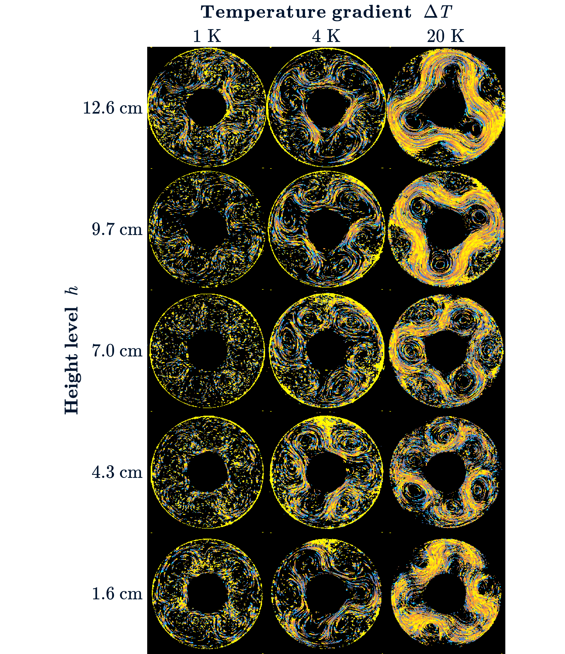
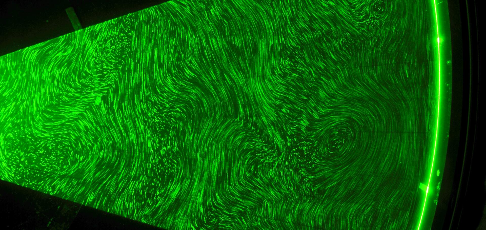
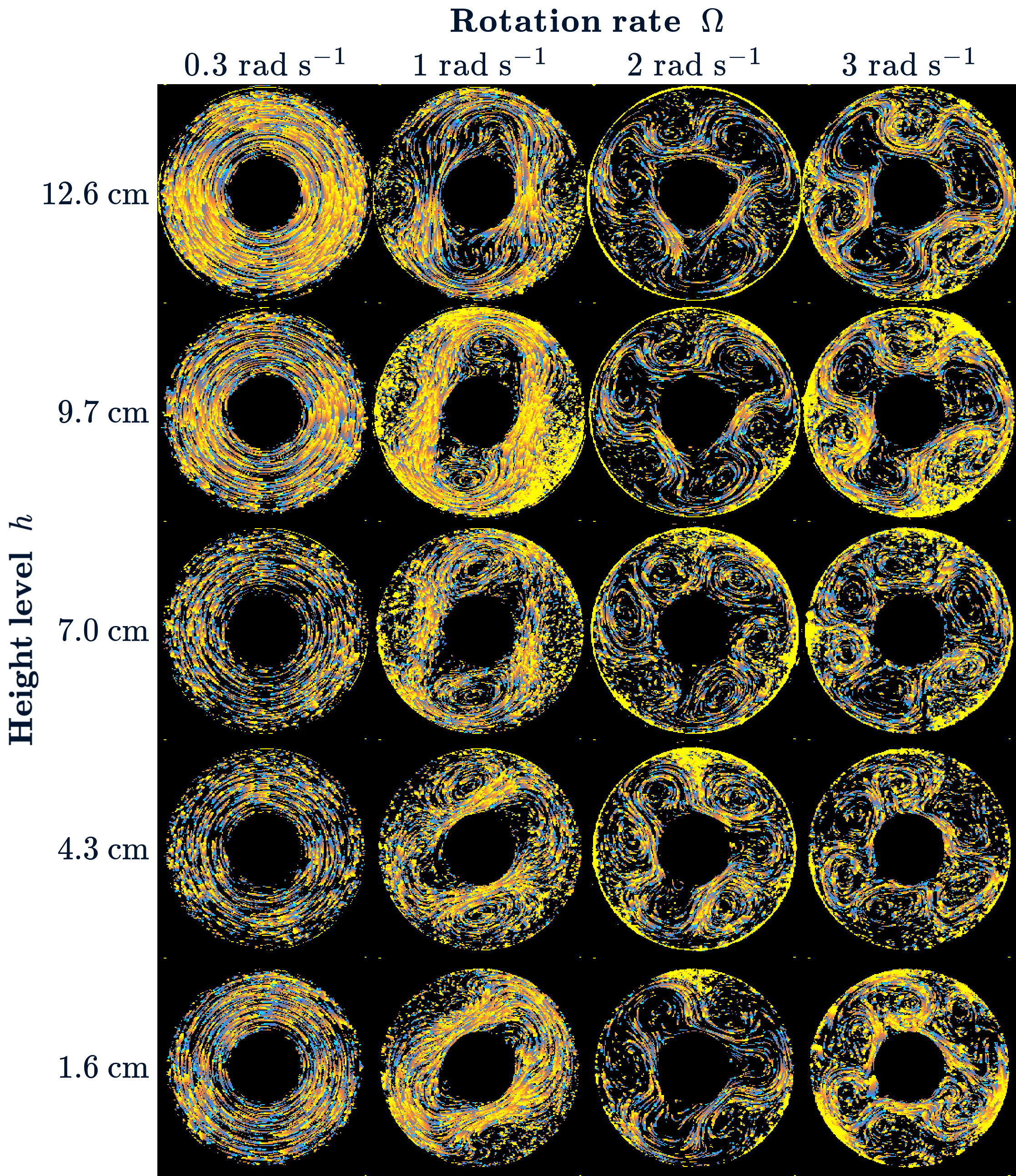
These features can also be seen in actual visualisations of baroclinic wave flows in the laboratory. The images below show some examples of streak visualisations at different heights within fully developed baroclinic wave flows under various conditions.
The properties of the annulus used for the streak images below are as follows:
- Inner radius: \(a=2.5\text{ cm}\)
- Outer radius: \(b=8.0\text{ cm}\)
- Height: \(d=14.0\text{ cm}\)
- Rigid lid
- Vertical axis of rotation
- Rotation rate: \(\Omega=0.05\text{ rad s}^{-1}\) to \(\Omega=4\text{ rad s}^{-1}\)
The following parameters are the same for each experiment:
- Density: \(1.050\text{ g cm}^{-3}\)
- Time interval between level switching: \(1\text{ min}\)
- Streak length: \(1\text{ s}\)
- Streaks change colour from orange at the leading end to blue at the trailing end.
Constant temperature gradient: \(\Delta T = 4\text{ K}\)
Constant rotation rate: \(\Omega = 2\text{ rad s}^{-1}\)