Tutorial 1.5
Baroclinic wave flows in a two-layer fluid
One of the earliest theoretical models for baroclinic instability, proposed in 1951 by Norman Phillips (Phillips 1951), simplified the vertical density stratification of the basic background flow by assuming two superposed, uniform layers of fluid of densities \(\rho_1\) (upper) and \(\rho_2\) (lower), such that the upper layer density is \(\rho_1 < \rho_2\) in a statically stable configuration – see Fig. 1.5a below. The initial flow consists of uniform zonal motion (in the \(x\)-direction) in each layer, with eastward flow \(u_1=+\frac{U}{2}\) in the upper layer and westward flow \(u_2=-\frac{U}{2}\) in the lower layer, along a straight channel of width \(L\) and total depth \(D\).
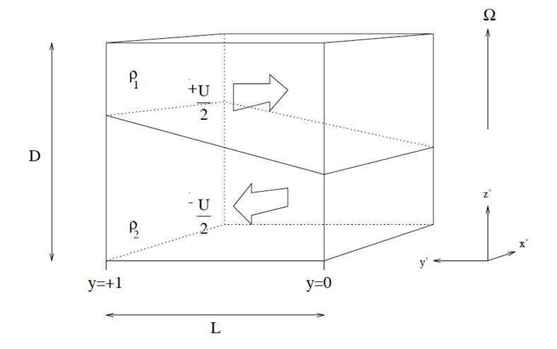
To maintain this flow in a steady state, in geostrophic balance with the background rotation speed \(\Omega\), the interface between the two layers must therefore slope upwards towards increasing \(y\) (northwards in the Northern Hemisphere). The slope of the interface must scale as \[\frac{\partial h_2}{\partial y} = \frac{2 \Omega}{g'}(u_1-u_2) = \frac{2 \Omega U}{g'}\] where \(g' = g \frac{\rho_2-\rho_1}{\rho_1}\) is the reduced gravity, thereby storing potential energy.
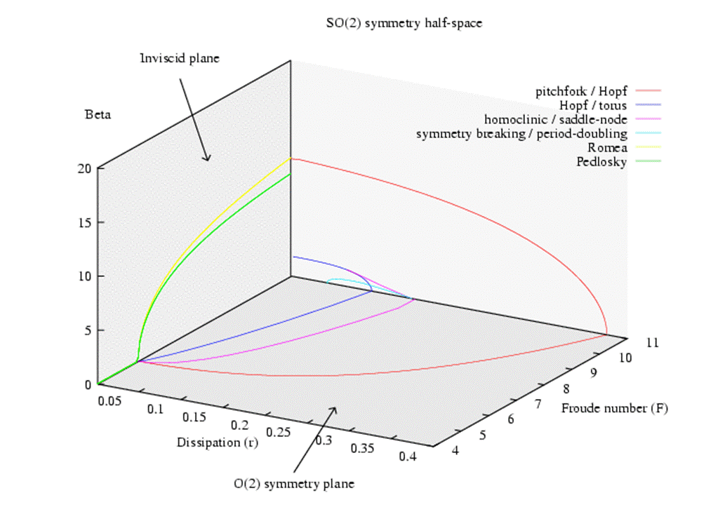
In principle, this potential energy can be released in the same way as in continuously stratified flows (see section 1), by the action of a wave-like baroclinic instability, provided that other dynamical constraints are satisfied. A more detailed model calculation, taking into account Ekman friction and the dependence of the Coriolis parameter \(f\) with latitude \(y\) (so \(f=f_0+\beta y\)), shows that the onset of baroclinic instability (and its nonlinear development) depend on three main dimensionless parameters:
- Froude number \[F=\frac{2 f_0^2 L^2}{g' D}\]
- Beta parameter \[B=\frac{\beta L^2}{U}\]
- Dissipation parameter \[r=\frac{\sqrt{2 v f_0} L}{U D}\]
The overall predicted regime diagram for this model is shown below (from Lovegrove et al. 2002):
This system is not just an abstract mathematical theory, however – it can be realised and explored in laboratory experiments. The figures below show a rotating annulus experiment that uses two immiscible fluids in uniform layers in a cylindrical annular tank. In practice, water was used as the upper layer and a mixture of an organic oil (D-Limonene) with a dense chlorofluorocarbon liquid (CFC-113) used for the lower layer, resulting in two layers with a density difference \(\Delta\rho=6\text{ kg m}^{-3}\), a mean density \(\bar{\rho}=1000\text{ kg m}^{-3}\), and reduced gravity \(g'=5.9\text{ cm s}^{-2}\).
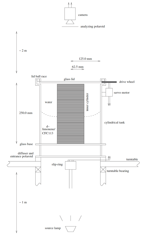
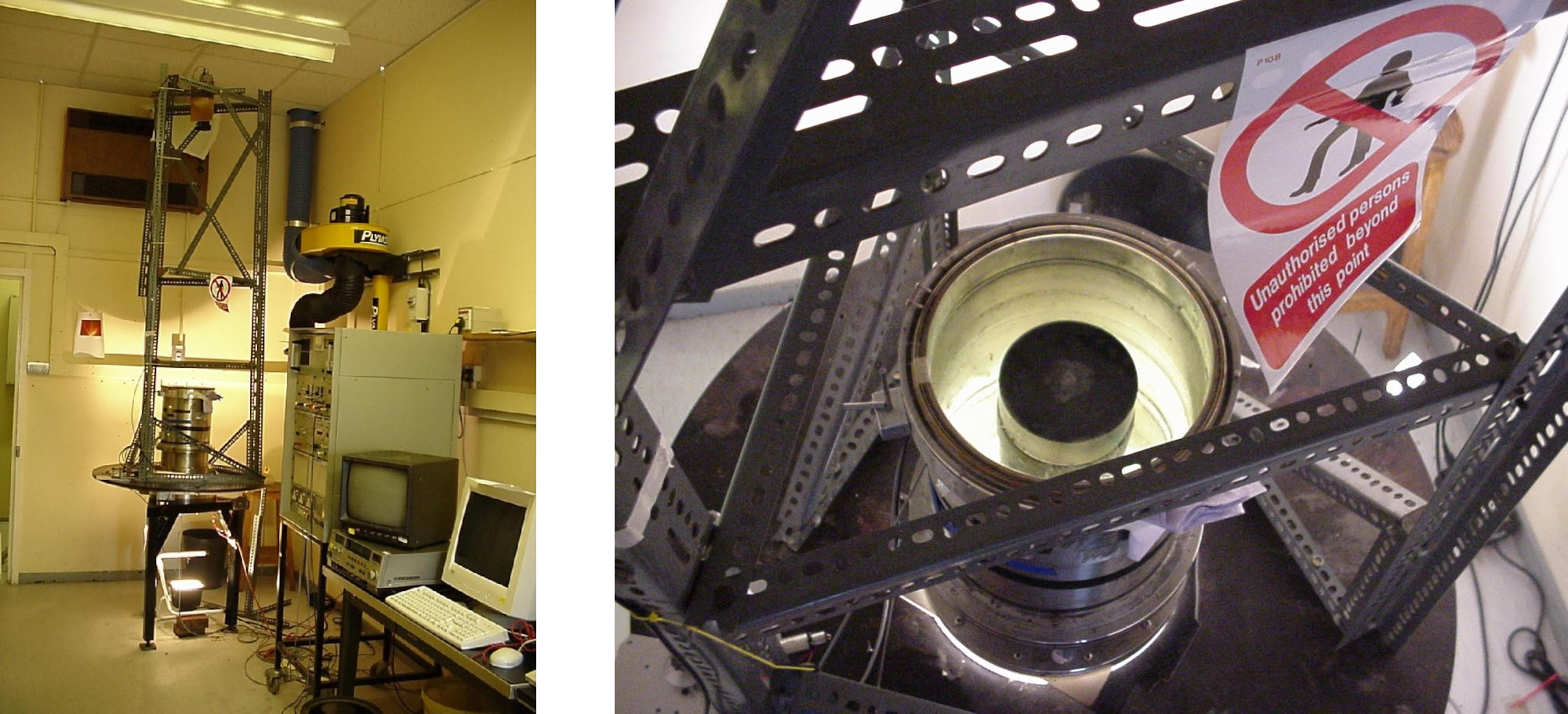
The differential zonal motion between the upper and lower layers is maintained mechanically by rotating the lid of the tank with respect to the rest of the tank (in either direction). The requirement for geostrophic balance leads to the interface between the layers becoming parabolically sloped in radius, as shown schematically above. When waves develop as a result of instabilities, these appear as wave-like perturbations to the interface in geostrophic balance with horizontal velocity perturbations in each layer.
We visualise these perturbations to the interface using a clever optical method, due originally to Hart & Kittleman 1985. The lower layer includes the material D-Limonene, an organic oil distilled from the peel of citrus fruits such as oranges or lemons. This is strongly optically active, which means it systematically rotates the plane of polarization of by an amount that depends on the optical path length and the wavelength of light. The variation of the angle of rotation at fixed optical path length is shown below, which clearly shows the strong wavelength dependence:

As indicated above, we shine white, plane polarized light upwards through the bottom of the tank through a neutral diffuser, towards a colour video camera located above the tank on the rotation axis. By adding a second polarising filter between the camera and the top of the tank, we allow only a single wavelength of light to come into alignment with the second polarizer for a given optical path length. But if the path length varies across the tank because of dynamical perturbations to the interface, different heights are mapped onto different colours!
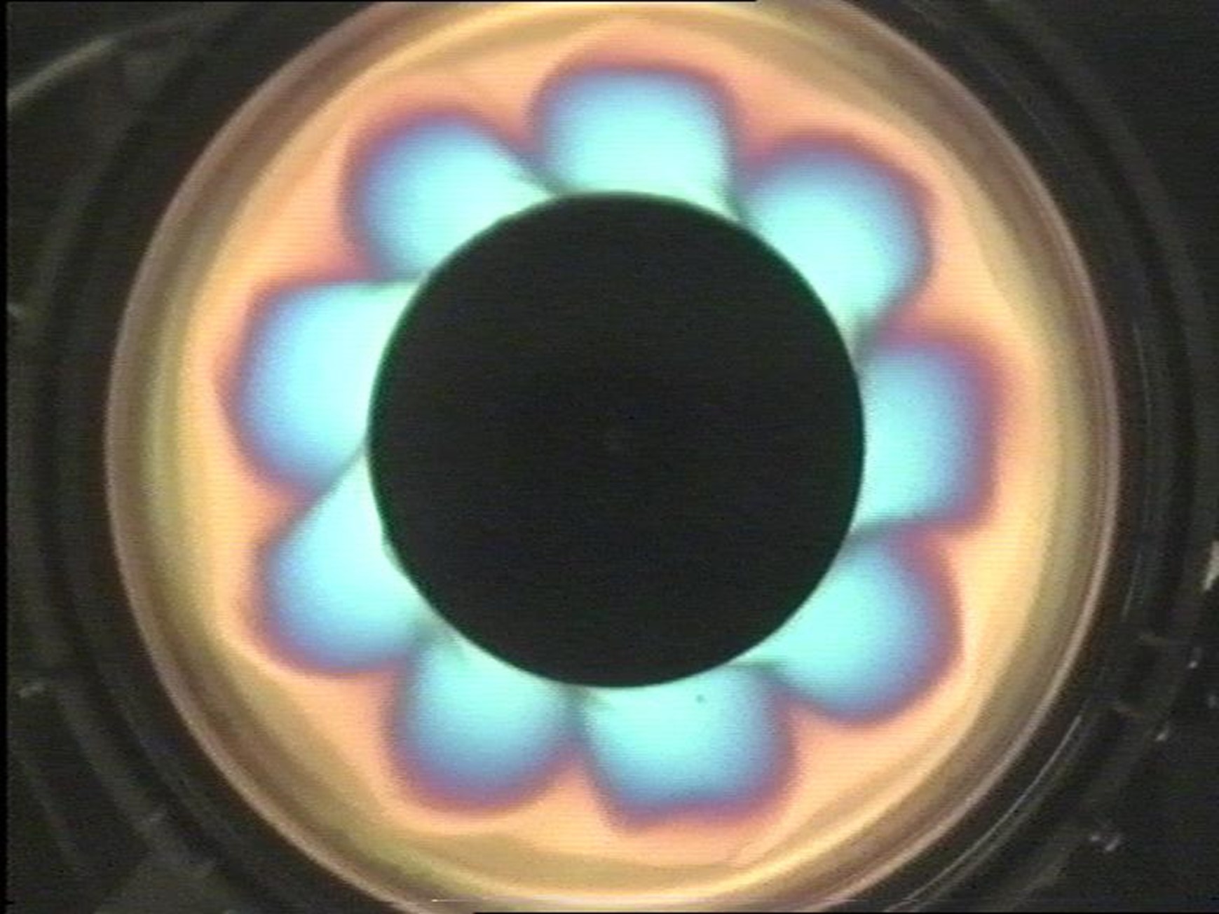
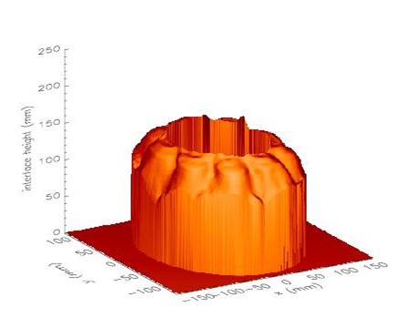
With care, the colour mapping can even be calibrated to recover a quantitative map of the interface, as shown above (from Williams et al. 2004).
This method can then be used to explore what kinds of flow may occur in different regions of parameter space, mainly with respect to the Froude number \(F\) and dissipation parameter \(r\).
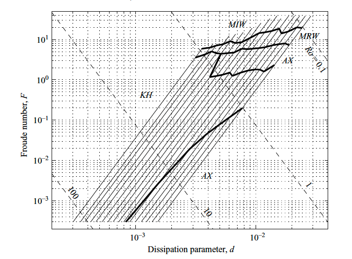
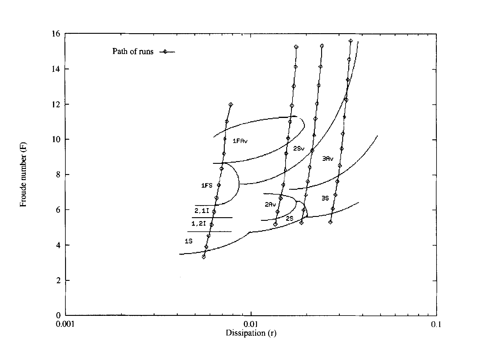
S: steady wave (apart from a slow drift around the annulus)
Av: periodic amplitude vacillation
Sv: structural vacillation
I: intermittent bursting flow
F: anomalous forced-resonant flow
Lists such as 2, 1I, etc. denote multiple equilibria.
Various flow regimes are indicated here, including:
AX: Axisymmetric flow
KH: Kelvin–Helmholtz shear instability (occurs when Richardson number \(\textrm{Ri}<0.25\) unless baroclinic instability is active)
MRW: mixed regular Wwves (steady or periodic baroclinic waves, mixed with the presence of short wavelength capillary-gravity waves)
MIW: mixed irregular waves (chaotic baroclinic waves, mixed with the presence of short wavelength capillary-gravity waves)
The movies below show examples of each of these regimes.