Home
Department Of Physics text logo
  • Research
    • Our research
    • Our research groups
    • Our research in action
    • Research funding support
    • Summer internships for undergraduates
  • Study
    • Undergraduates
    • Postgraduates
  • Engage
    • For alumni
    • For business
    • For schools
    • For the public
  • Support
Menu
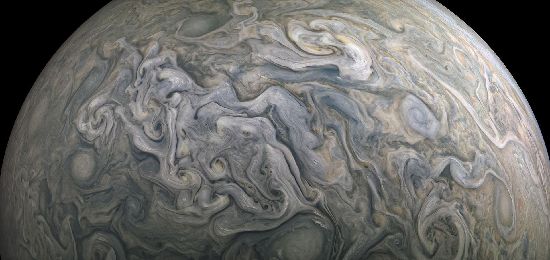
Juno Jupiter image

Prof. Patrick Irwin

Professor of Planetary Physics

Research theme

  • Exoplanets and planetary physics

Sub department

  • Atmospheric, Oceanic and Planetary Physics

Research groups

  • Exoplanet atmospheres
  • Planetary atmosphere observation analysis
  • Solar system
patrick.irwin@physics.ox.ac.uk
Telephone: 01865 (2)72083
Atmospheric Physics Clarendon Laboratory, room 306
Personal research page
NEMESIS
Github data sharing website
  • About
  • Publications

A calibrated Cassini/VIMS catalog of Jupiter spectral cubes from the 2000–2001 flyby

(2026)

Authors:

Asier Anguiano-Arteaga, Patrick Irwin, Santiago Pérez-Hoyos, Davide Grassi, Emiliano D'Aversa

Abstract:

Cassini observed Jupiter during its 2000–2001 gravity-assist flyby, acquiring a valuable set of Visible and Infrared Mapping Spectrometer (VIMS) observations over a wide range of viewing geometries and observing conditions. These data comprise visible and infrared spectral cubes covering the VIS channel from 0.35 to 1.05 µm and the IR channel from 0.9 to 5.1 µm. We present a calibrated catalog of these Jupiter VIMS observations,  excluding satellite-targeted observations, designed to provide a homogeneous and validated set of spectral products for future Jovian studies.Starting from the raw archive cubes, we developed a processing workflow that combines ISIS/SPICE-based geometry recovery with dedicated radiometric calibration procedures for both VIMS channels. The final products are delivered as multi-extension FITS files containing calibrated I/F spectral cubes, wavelength and FWHM vectors, and geometry backplanes for incidence, emission, and phase angles, planetocentric latitude, positive-east longitude, pixel resolution, and azimuth angle. The workflow also addresses several issues affecting the original data set, including saturation, VIS pointing-related offsets between radiometric cubes and geometric backplanes, channel-dependent dark-signal artifacts, and a subset of IR approach-phase for which the standard ISIS calibration pipeline can produce over-scaled reflected spectra.The resulting catalog provides a uniform, documented, validated, and publicly available set of Cassini/VIMS Jupiter products. By combining calibrated VIS and IR cubes with wavelength information and geometry backplanes, these products facilitate a wide range of applications in the study of Jupiter and its atmosphere.
More details from the publisher

Cold Temperatures, Dark Clouds, or Missing Absorption: What Does the 5-Micron Window Tell Us about the Ice Giants?

(2026)

Authors:

Michael Roman, Leigh Fletcher, Oliver King, Simon Toogood, Heidi Hammel, Patrick Irwin, Joseph Penn, Imke de Pater, Henrik Melin, Stefanie Miliam

Abstract:

JWST-NIRSpec observations are providing our first detailed view of the Ice Giants in the 5-micron spectral window [1]. Observations of Jupiter and Saturn (see Figure) at 5 microns have historically revealed important insights into their tropospheric composition, along with striking images of clouds silhouetted against the glowing thermal emission from deeper atmospheric layers [2]. Comparable observations of the colder Ice Giants, however, have long remained beyond observational reach—until now.In this talk, we present JWST-NIRSpec 5-micron observations of the Ice Giants and discuss their implications. We examine what these observations reveal about the tropospheric temperatures, clouds, and composition of Uranus and Neptune, as well as what they may imply for current radiative transfer models at these wavelengths.In particular, we find that the JWST data may suggest sub-adiabatic temperature gradients near the cloud layers, resulting in colder temperatures in the deeper atmosphere. However, these conclusions depend sensitively on the scattering properties of Ice Giant clouds and on accurate modelling of the gaseous opacity, both of which, we argue, remain uncertain under these conditions.Figure: Saturn at 5 microns (left, in red) from Cassini, with hazes shown in green (Image credits: NASA/JPL-Caltech/University of Arizona), compared to Uranus at 5 microns from JWST-NIRSpec [1].[1] Roman, M.T., et al., The Infrared Spectrum of Uranus Revealed with JWST (submitted)[2] Wong, M.H., Bjoraker, G.L., Goullaud, C., Stephens, A.W., Luszcz-Cook, S.H.,1047Atreya, S.K., Pater, I., Brown, S.T.: Deep clouds on jupiter. Remote Sensing104815(3), 702 (2023) 
More details from the publisher

Decomposing Titan’s far-infrared Haze B feature with PCA and NMF analysis

(2026)

Authors:

Joshua S Ford, Nicholas A Teanby, Patrick GJ Irwin, Conor A Nixon, Lucy Wright

Abstract:

During its flyby of Titan in 1980, Voyager 1 unveiled an atmosphere thick with an opaque, orange haze that completely obscured the surface, and provide  the first close-up images of its vertical layering (Smith et al. 1981, Hanel et al 1981). Subsequent observations from the Cassini-Huygens mission (Flasar et al. 2004) expanded this view, revealing a world dominated by photochemical hydrocarbons and nitriles with lakes of methane  (Stofan et al. 2007, Mastrogiuseppe et al. 2019), tholin-like organic sand (Lorenz et al. 2006), and seasonally evolving ice clouds (Jennings et al. 2012, West et al. 2016) as seen in Figure 1. While recent observations and laboratory studies (Anderson et al. 2011, Chatain et al. 2020) have provided greater insights into the physical properties of these aerosols and how they form, their composition and complexity remain a mystery.Figure 1: Image taken by Cassini Imaging Science Subsystem (Credit: NASA/JPL-Caltech/Space Science Institute) showing a large ice cloud possibly made of HCN at 300km in Titan’s south pole, 2012 (West et. 2016, Vinatier et al. 2018)In the upper atmosphere, nitrogen and methane are photodissociated by UV radiation and energetic particles to produce ions which act as embryos for the growth of large organic molecules (Vuitton et al. 2024). As these molecules sink through the atmosphere, they recombine, coagulate, and accumulate into larger aerosol particles, onto which trace species can condense, forming both photochemical hazes and stratospheric ice clouds (Vuitton et al. 2024). Cassini CIRS (Composite Infrared Spectrometer) far infra-red spectra (FP1) exhibit four types of hazes: Haze 0, Haze A, Haze B (otherwise known as the “Haystack”) and Haze C (de Kok et al. 2007). While Haze 0 is present throughout the CIRS spectral range and affects the spectral continuum, Haze A, B and C appear as broad features in the far-infrared range. Relatively little is known about these hazes, making their features difficult to fit and estimate. In addition, their signatures overlap with H2O, C4H2, C2N2 and CH4 rotational lines, complicating retrievals of these gases (Sylvestre et al.2017).  Among these hazes, Haze B exhibits the strongest spectral signature. Anderson et al. 2018 suggested that the composition must be a mixture of more than one chemical compound due to its magnitude, breadth and opacity. Haze B is observed to only be present at the winter poles, forming and dissipating with the changing seasons, most likely caused by reduced sunlight and temperature (Jennings et al. 2012a,b , Anderson et al 2018).To enable accurate fitting of water features, Ford et al. (in review) retrieved an effective spectral cross-section of Cassini CIRS FP1 spectra between 147-257cm-1 of 156 FIRNADCMP 0.5cm-1 observations (Figure 2) across different latitudes and times (see also Ford et al. 2025). This was achieved by scaling gaussian basis functions to fit Haze A, B and C (and any other unknown aerosols) in the spectra baselines using the NEMESIS radiative transfer code (Irwin et al. 2008). Previous aerosol cross-sections did not account for latitude or time variation and therefore this technique empirically and agnostically modelled the changing baseline.  In this study, we decomposed those 156 effective spectral cross-sections and extrapolated unique Haze B cross-sections for latitudes of -89° to 88° from June 2004 to April 2017.  We used principal component analysis to determine the number of complete hazes present in the spectral range, finding that Haze B accounts for 98% of the observed variation. We then applied non-negative matrix factorisation to seperate the spectra into two unique and stable components: one representing Haze B, and a second representing a mixture of other haze contributions, along with numerical and spectral noise.Figure 2: Effective spectral cross-section of all 156 Cassini CIRS FIRNADCMP 0.5cm-1 observations before decomposition. Each colour represents a different observation. The plot shows the variation extent of the Haze B feature at ~220cm-1. Using the maximum Haze B cross-section of each observation as proxy, we find a large increase at the winter poles with the increase during northern spring being nearly twice that of northern winter, consistent with previous investigations. We also find Haze B extends to 60°, different to 70° proposed by Anderson et al. 2018. The results also give an insight into the time of formation/dispersion of Haze B at the poles. We see that Haze B at the south pole forms around 2013, reaching its peak during the summer solstice. The final dissipation of Haze B at the north pole cannot be determined due to limited data. ReferencesAnderson, C.M. et al. (2011), Icarus,  212.2, 762-778. DOI: 10.1016/j.pss.2010.10.009Anderson, C.M. et al. (2018), Organic Ices in Titan’s Stratosphere in Space Science Reviews, 214.8, 125  DOI: 10.1007/s11214-018-0559-5Chatain, A.  et al. (2020), Icarus, 345, 113741. DOI: 10.1016/j.icarus/2020.113741Coustenis, A. et al. (1999), Planet Space Science, 47, 1305-1329. DOI:  10.1016/S0032-0633(99)00053-7de Kok, R. et al. (2007), Icarus, 191, 223. DOI:10.1016/j.icarus.2007.04.003Flasar, F.M. et al. (2004), Space Science Reviews, 115, 169–297. DOI: 10.1007/s11214-004-1454-9Ford, J.S. et al. (2025),  EGU General Assembly 2025, Vienna, Austria, EGU25-3741. DOI: 10.5194/egusphere-egu25-3741Ford, J.S. et al. In review. Titan’s Stratospheric Water: Latitudinal and Seasonal Variation from Cassini CIRS Data and Implications for External Oxygen Sources. PSJHanel, R.A. et al. (1981), Science, 212, 192–200. DOI: 10.1126/science.212.4491.192Irwin, P.G.J et al. (2008), JQSRT, 109, 1136. DOI: 10.1016/j.jqsrt.2007.11.006Jennings, D.E. et al. (2012), The Astrophysical Journal Letters, 754, L3. DOI: 10.1088/2041-8205/754/1/L3Khanna, R.K. (2005), Icarus, 178,165-170. doi:10.1016/j.icarus.2005.03.011Lorenz, R. et al. (2006), Science, 312, 724–727. DOI: 10.1126/science.1123257Mastrogiuseppe, M. et al. (2019), Nature Astronomy, 3, 535, DOI: 10.1038/s41550-019-0714-2Samuelson, R.E. Clouds and aerosols of Titan’s atmosphere, in The Atmospheres of Saturn and Titan. Proc.Int. Workshop, vol. ESA SP-241 (1985)Smith, B.A. et al. (1981), Science, 212, 163–191. DOI: 10.1126/science.212.4491.163Stofan, E.R. et al. (2007), Nature, 445, 61–64. DOI: 10.1038/nature05438Sylvestre, M. et al. (2017), A&A, 609:A64. DOI: 10.1051/0004-6361/201630255Vinatier, S. et al. (2018),  Icarus, 310, 89-104. DOI: 10.1016/j.icarus.2017.12.040Vuitton, V. et al. (2024), Chapter 6:Titan’s Atmospheric Structure, Composition, Haze, and Dynamics in Titan after Cassini–Huygens, COSPAR Scientific Symposium Series.West, R.A. et al, (2016), Icarus, 270, 399-408. DOI: 10.1016/j.icarus.2014.11.038 
More details from the publisher

Final results: Jovian upper clouds and hazes from visible and near infrared spectroscopy using CARMENES

(2026)

Authors:

José Ribeiro, Pedro Machado, Santiago Pérez-Hoyos, Asier Anguiano-Arteaga, Patrick Irwin

Abstract:

The origin and vertical distribution of Jupiter’s red coloration remain uncertain, despite multiple proposed aerosol models. Laboratory work (Carlson et al., 2016) showed that photolyzed ammonia and acetylene can form a red compound consistent with Jupiter’s colours, motivating the “universal chromophore” hypothesis (Sromovsky et al., 2017), and the “Crème Brûlée” model (Baines et al., 2019), which places a thin absorber above the ammonia clouds. Later HST and VLT studies (Pérez‑Hoyos et al., 2020; Braude et al., 2020) suggested a more vertically extended, less blue‑absorbing material, while recent analyses of the Great Red Spot and Oval BA indicate the presence of two distinct colouring agents: a universal‑chromophore absorber and a deeper UV‑absorbing aerosol (Anguiano‑Arteaga et al., 2021, 2023). These findings highlight persistent ambiguity in Jovian aerosol composition and structure.To investigate this, we analysed 2019 Jupiter observations from CARMENES (The Calar Alto High-Resolution search for M dwarfs with Exoearths with Near-infrared and optical Échelle Spectrographs), (0.52–1.71 μm). Since no calibration star was available, we calibrated the spectra using Saturn’s B ring and Cassini/VIMS reflectivity (Cuzzi et al., 2009), achieving agreement with published Jupiter spectra to within 10% (Clark, R.N., McCord, T.B., 1979; Mendikoa, I., et al., 2017; Irwin, P.G., et al., 2018).Using 64 VIS–NIR observation pairs, we performed a Minnaert limb‑darkening analysis and generated synthetic spectra for five regions. These were used in NEMESIS retrievals with three aerosol models. Across all models, the highest‑altitude aerosol layer dominated the spectral behaviour, with particle size, cloud‑base abundance, and pressure level strongly influencing the fits. Model B (Braude et al., 2020) produced the lowest χ²/Nfree values, but no model fully reproduced the observations, likely due to the limited wavelength range, which lacks constraints on deeper clouds.The models diverged in retrieved particle sizes and cloud‑base pressures, with several results, such as extremely small tropospheric particles or overly large stratospheric particles, indicating physical inconsistencies. Model A’s tropospheric haze base aligns with Galileo probe measurements (Sromovsky and Fry, 2002); Model C retrieves a cloud base level near the NH₄SH level predicted by Atreya (1998), deeper than CIRS detections (Matcheva et al.,2005) but within the range of Baines et al. (2019), with implausible particle sizes.Overall, the study shows that CARMENES can deliver high‑quality, flux‑calibrated planetary spectra, but also that broader spectral coverage is essential to resolve Jupiter’s chromophore composition and aerosol vertical structure. Figure 1: Location of the spectra used to perform the Minnaert limb-darkening approximation for each region considered in this study. Red for EZ, yellow for NEB, green for SEB, pink for SEB transition and blue for NEB transition. The Jupiter AGC image represented corresponds only to the spectra of the EZ whose longitude was closest to 0º. Figure 2: Comparison between observed and modelled spectra and residuals for EZ using model B]{Comparison between observed (blue) and modelled (red) spectra (left column) and comparison between differences (red) and a priori errors (black) (right column) for the EZ using model B, with the grey shaded areas corresponding to telluric absorption. The top row corresponds to nadir (incidence and emission angle = 0º) and the bottom row to limb (incidence and emission angle = 61.45º). Figure 3: Comparison between the a priori aerosol vertical profiles and the retrieved profiles for every region for models A and B. We compare the optical depth/atm at 0.90 μm of model B with all three aerosol populations considered and model A's stratospheric and tropospheric hazes. The horizontal dashed line corresponds to 0.15 atm, separating model B's deep cloud layer from the haze. References:Carlson, R. W., et al. (2016). Chromophores from photolyzed ammonia reacting with acetylene: Application to Jupiter's Great Red Spot. Icarus, 274, 106–115.Sromovsky, L. A., et al. (2017). A possibly universal red chromophore for modeling color variations on Jupiter. Icarus, 291, 232–244.Baines, K. H., et al. (2019). The visual spectrum of Jupiter's Great Red Spot accurately modelled with aerosols produced by photolyzed ammonia reacting with acetylene. Icarus, 330, 217–229.Pérez-Hoyos, S., et al. (2020). Color and aerosol changes in Jupiter after a North temperate belt disturbance. Icarus, 132, 114021.Braude, A. S., et al. (2020). Colour and tropospheric cloud structure of Jupiter from MUSE/VLT: Retrieving a universal chromophore. Icarus, 338, 113589.Anguiano-Arteaga, A., et al. (2021). Vertical Distribution of Aerosols and Hazes Over Jupiter's Great Red Spot and Its Surroundings in 2016 From HST/WFC3 Imaging. Journal of Geophysical Research: Planets, 126, e2021JE006996.Anguiano-Arteaga, A., et al. (2023). Temporal variations in vertical cloud structure of Jupiter's Great Red Spot, its surroundings and Oval BA from HST/WFC3 imaging. Journal of Geophysical Research: Planets, 128, e2022JE007427.Irwin, P., et al. (2008). The NEMESIS planetary atmosphere radiative transfer and retrieval tool. J. Quant. Spectrosc. Radiat. Transf., 109, 1136–1150.Rodgers CD. (2000). Inverse methods for atmospheric sounding: theory and practice. Singapore: World Scientific.Cuzzi, J., et al., 2009. Ring Particle Composition and Size Distribution. Springer Netherlands, Dordrecht. pp. 459–509.Clark, R.N., McCord, T.B., 1979. Jupiter and Saturn: Near-infrared spectral albedos. Icarus 40, 180–188.Mendikoa, I., et al., 2017. Temporal and spatial variations of the absolute reflectivity of Jupiter and Saturn from 0.38 to 1.7 𝜇m with planetcam-upv/ehu. A&A 607, A72.Irwin, P.G., et al., 2018. Analysis of gaseous ammonia (NH3) absorption in the visible spectrum of Jupiter. Icarus 302, 426–436.Matcheva, K.I., Conrath, B.J., Gierasch, P.J., Flasar, F.M., 2005. The cloud structure of the jovian atmosphere as seen by the Cassini/CIRS experiment. Icarus 179(2), 432–448.Sromovsky, L., Fry, P., 2002. Jupiter’s cloud structure as constrained by Galileo probe and HST observations. Icarus 157 (2), 373–400.
More details from the publisher

H2S Cloud Properties in Uranus and Neptune: Sensitivity to Deep Composition and Vertical Mixing

(2026)

Authors:

Daniel Toledo, Pascal Rannou, Patrick Irwin, Michael Roman, Bruno de Batz de Trenquelléon, Raul Rodriguez-Veloso, Clara Lorenzo-Corvo, Víctor Apéstigue, Marco Personat, Ignacio Arruego

Abstract:

Radiative transfer analyses of Uranus and Neptune spectra have revealed a cloud layer at pressures greater than ~2 bar (1,2), with H₂S gas detected above it on both planets (3,4), suggesting H₂S ice as its main constituent. However, the properties of these clouds and their dependence on the deep atmospheric composition remain poorly constrained.We present an extended version of a one-dimensional cloud microphysics model [5,6] previously applied to simulate CH₄ and H₂S clouds in the Ice Giants (7,8). The model now incorporates NH₄SH chemistry, extending the simulation domain to ~50 bar. Since NH₃ reacts with H₂S to form NH₄SH at depth, the deep N/S ratio controls how much H₂S is available to condense at higher altitudes. We explore how the deep NH₃ and H₂S abundances, together with the vertical mixing profile, determine the properties of the H₂S cloud layer, including its base pressure, total opacity, and particle size distribution.Preliminary results and the implications of this work for the interpretation of current and future observations of Uranus and Neptune will be discussed.References: [1] P. G. Irwin, et al., JGR: Planets, 127, e2022JE007189. [2] L. Sromovsky, et al., Icarus,Volume 317, (2019) [3] P. G. Irwin, et al., Nature Astronomy 2, 420 (2018). [4] P. G. Irwin, et al., Icarus 321, 550 (2019). ). [5] P. Rannou, et al., Science 311, 201 (2006). [6] F. Montmessin, et al., JGR: Planets 107, 4 (2002). [7] D. Toledo, et al., A&A, 694, A81 (2025). [8] D. Toledo, et al.,: Microphysical Modeling of Hydrogen Sulfide Clouds in the Atmospheres of the Ice Giants, EPSC-DPS Joint Meeting 2025,  https://doi.org/10.5194/epsc-dps2025-1456, 2025.
More details from the publisher

Pagination

  • First page First
  • Previous page Prev
  • Page 1
  • Current page 2
  • Page 3
  • Page 4
  • Page 5
  • Page 6
  • Page 7
  • Page 8
  • Page 9
  • …
  • Next page Next
  • Last page Last

Footer Menu

  • Contact us
  • Giving to the Dept of Physics
  • Work with us
  • Media

User account menu

  • Log in

Follow us

FIND US

Clarendon Laboratory,

Parks Road,

Oxford,

OX1 3PU

CONTACT US

Tel: +44(0)1865272200

University of Oxfrod logo Department Of Physics text logo
IOP Juno Champion logo Athena Swan Silver Award logo

© University of Oxford - Department of Physics

Cookies | Privacy policy | Accessibility statement

Built by: Versantus

  • Home
  • Research
  • Study
  • Engage
  • Our people
  • News & Comment
  • Events
  • Our facilities & services
  • About us
  • Giving to Physics
  • Current students
  • Staff intranet