Comparative study of the retrievals from Venera 11, 13, and 14 spectrophotometric data.
(2025)
Abstract:
Deconvolution and Data Analysis Tools Applied to GEMINI/NIFS Archival Data Enables Further Constrains on H2S Abundance in Neptunes Atmosphere
Copernicus Publications (2025)
Abstract:
We present a re-analysis of archival data-cubes of Neptune obtained with the GEMINI Near-Infrared Integral Field Spectrometer (NIFS), aiming to refine constraints on the abundance of hydrogen sulphide (H₂S) in Neptune's atmosphere. To enhance spatial and spectral fidelity, we employ a modified CLEAN algorithm that effectively deconvolves the data while conserving flux. To mitigate observational and instrumental artifacts, we utilize Singular Spectrum Analysis (SSA) on single-wavelength images and apply Principal Component Analysis (PCA) across the full data-cube to suppress both random and systematic noise. Spectral retrievals are conducted using ArchNemesis, an optimal estimation inverse modeling tool. We retrieve vertical profiles at individual locations, and use Minnaert-corrected reflectivity functions across latitude bands to investigate latitudinal variability. Using the deconvolution and data analysis techniques, we are able to extract more scientific utility from legacy datasets and describe a template that can be repeated for similar datasets.Improving cloud microphysical parametrizations for ultra-hot Jupiter TOI-1431b
Copernicus Publications (2025)
Abstract:
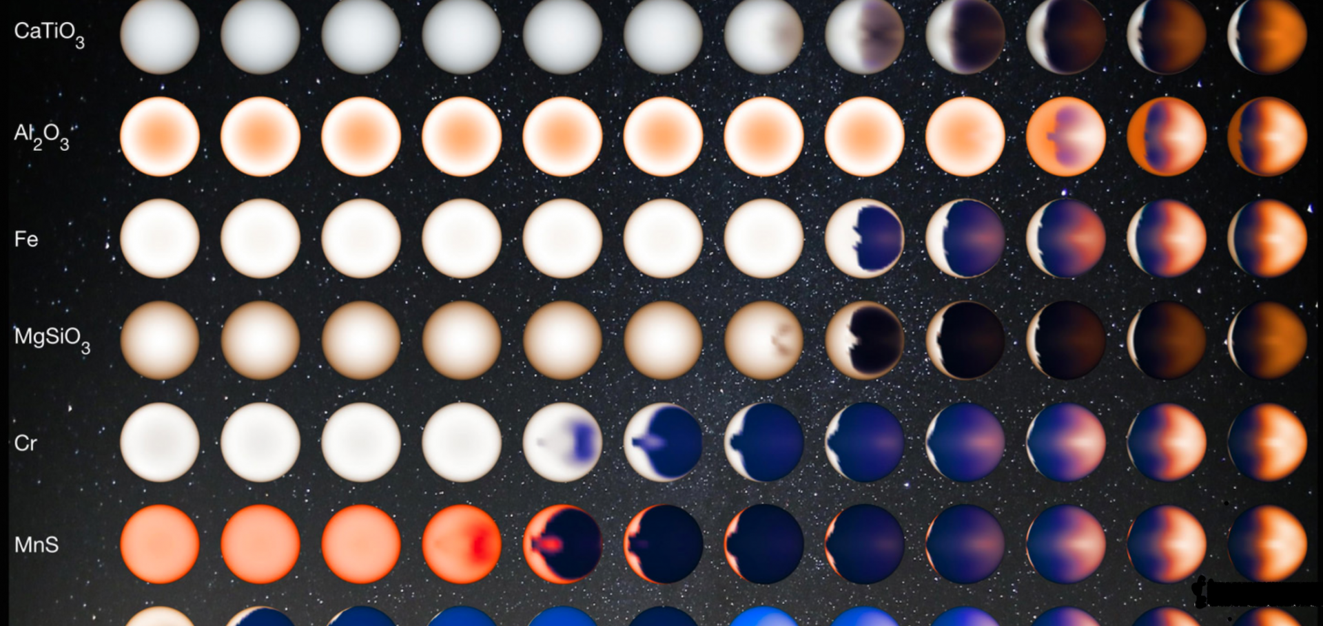
Clouds have broad significance in understanding the evolution and climate of planetary atmospheres. Moreover, the presence of clouds in the atmospheres of hot Jupiter exoplanets is supported both by direct spectral detections (Grant et al. 2023, Inglis et al. 2024), and observational trends, such as nightside brightness temperature (Beatty et al. 2019) and phase curve hot spot offsets (Bell et al. 2024), suggesting that an accurate understanding of clouds is needed, not only to understand the atmospheres of these planets, but to properly interpret observations. However, the properties of clouds are impacted by inherently coupled effects of circulation, radiation, and cloud microphysics. Full coupling of these processes remains computationally expensive, and as a result, current modeling schemes implement simplified cloud parametrizations that neglect one or more of these effects. Within this work, we implement a one-way indirect coupling of the cloud microphysical model 1D CARMA and MITgcm/DISORT, a general circulation model including double-grey radiative transfer, through including a novel particle size distribution that better represents the output of CARMA. We use pre-existing CARMA data for ultra-hot Jupiter TOI-1431b from Gao & Powell (2021), which has particle size distributions that are not well described by a log-normal distribution, with corundum in particular displaying distinctly bimodal behavior. We hypothesize the smaller particle size mode corresponds to nucleation, whereas the larger particle size has formed through condensational growth and coagulation. We present a particle size distribution function that can account for this wide range of distribution variability using two log-normals and two log-exponentials. We implement this particle size distribution for corundum within MITgcm/DISORT for ultra-hot Jupiter TOI-1431b, and compare this work to that of Komacek et al. (2022a), which includes a log-normal roughly corresponding with the larger particle size mode in our distribution. We present the results of this comparison, and discuss the impact of particle size distribution on properties of ultra-hot Jupiters.Investigating the Vertical Variability of Titan’s 14N/15N in HCN
(2025)
Abstract:
Jovian chromophore and upper hazes from CARMENES spectra
(2025)