The Latitudinal Variation of H2S Humidity on Uranus

Copernicus Publications (2026)

Authors:

Joseph Penn, Patrick Irwin, Jack Dobinson

Abstract:

The spectral signature of hydrogen sulphide (H2S) above the cloud tops in Uranus’ atmosphere was detected in 2018 [1]. The H2S humidity can be used as a tracer of Uranus’ overturning circulation [2] - peaks and troughs in the latitudinal humidity distribution may correspond to regions of local upwelling and downwelling near the H2S condensation level. We analysed observations from Gemini-NIFS and VLT-SINFONI, taken between 2009 and 2014, to study the H2S humidity distribution of Uranus. In our previous analysis of H2S on Neptune [3], we found a significant degeneracy between the methane (CH4) and H2S distributions, so we prescribe a latitudinally varying deep methane abundance previously derived from HST-STIS spectra [4]. We deconvolve the observations and extract spectra using the Minnaert limb-darkening approximation, which has been applied in several analyses of Ice Giant observations [3,4,5]. We fit a parameterised aerosol model and the H2S humidity to our extracted spectra with nested sampling using our open-source radiative transfer code, archNEMESIS [6]. Our atmospheric model has a large number of parameters, and to make nested sampling computationally feasible we utilise a trained neural network for early exploration of the parameter space during our retrievals. Since our observations span several years, we search for temporal changes. We find changes in the aerosol structure and aerosol spectral properties corresponding to the development of Uranus' north polar hood, in agreement with previous work [4,8]. If we assume that the CH4 distribution is stable over time, then our results show no significant changes in the H2S distribution.  Our results show a general equator-to-pole decrease in the H2S humidity, similar to what has been found in microwave analyses that are sensitive to the deep H2S distribution [7]. Superimposed on this are local increases, which are fairly evenly spaced in latitude. We found a somewhat similar pattern in our analysis of H2S on Neptune [3], and an analysis of Neptune with VLT/MUSE also found peaks in reflectivity with a similar spacing [5]. These results are suggestive of a complex circulation pattern near the deep H2S aerosol layer. [1] Irwin, P. G. J., et al. (2018). Detection of hydrogen sulfide above the clouds in Uranus's atmosphere. Nature Astronomy, 2(5), 420-427. [2] Fletcher, L.N., et al. (2020). Ice Giant Circulation Patterns: Implications for Atmospheric Probes. Space Sci Rev 216, 21[3] Penn, J., et al. (2026). Reconciling Near-Infrared and Microwave Analyses of Neptune’s Hydrogen Sulphide Distribution. Monthly Notices of the Royal Astronomical Society, 548, 2, [4] James, A., et al. (2023). The Temporal Brightening of Uranus' Northern Polar Hood From HST/WFC3 and HST/STIS Observations. Journal of Geophysical Research: Planets, 128(10), e2023JE007904.[5] Irwin, P. G. J., et al. (2023). Latitudinal Variations in Methane Abundance, Aerosol Opacity and Aerosol Scattering Efficiency in Neptune's atmosphere determined from VLT/MUSE. Journal of Geophysical Research: Planets, 128(11), e2023JE007980.[6] Alday, J., et al. (2025). archNEMESIS: An Open-Source Python Package for Analysis of Planetary Atmospheric Spectra. Journal of Open Research Software, doi:10.5334/jors.554.[7] Molter, E. M., et al. (2021). Tropospheric Composition and Circulation of Uranus with ALMA and the VLA. The Planetary Science Journal, 2(1), 3.[8] Sromovsky, L. A., et al. (2024). The puzzling north polar region of Uranus: Continued zero-shear winds and increasing brightness from 2015 through 2022 according to 7 years of Keck AO imaging. Icarus, 420, 116186.

Time-variability and north pole enhancement of Titan’s atmospheric water abundance 

(2026)

Authors:

Joshua S Ford, Nicholas A Teanby, Conor A Nixon, Patrick GJ Irwin, Veronique Vuitton, Lucy Wright

Abstract:

IntroductionOxygen is the universes third most abundant element (Bergman et al. 2021) and is extremely rich in the Saturnian system (Feuchtgruber et al. 1997). Studies have found oxygen-bearing molecules and ions in Saturn’s atmosphere (Esposito et al. 2005) , in its plasma environment (Wilson et al. 2016) and on its moon Enceladus (Thomas et al. 2016). In contrast, Titan is scare in oxygen species, boasting a rich atmosphere of hydrocarbons and nitriles (Vuitton et al.2024) that interact uniquely, often consuming free oxygen or locking it away as water ice. This results in an anoxic, organic and diverse environment with little oxygen to terminate reactions (Nixon et al. 2024).To date, only three oxygen-bearing molecules have been detected in Titan’s atmosphere: CO (Lutz et al. 1983), CO2 (Sameulson et al 1983) and H2O (Coustenis et al. 1997). These molecules form from externally delivered OH, O+  and/or H2O being photodissociated by solar UV and energetic particles in the upper atmosphere, before recombining and being transported downwards via atmospheric mixing (Vuitton et al. 2019).  Of the detected species, the least well-understood is water vapour. CO and CO2 have been studied extensively and exhibit little variation in latitude, time or altitude (Teanby et al. 2019). Yet, investigations into H2O have been limited to single measurements or large averages (Vuitton et al 2007,  Cui et al 2009, Cottini et al. 2012, Bauduin et al 2018). Its weak infrared emission lines and low atmospheric abundances make it difficult to model. Water plays a vital role in Titan’s atmosphere, distributing oxygen and acting as a tracer for atmospheric dynamics. Its chemical pathways may produce species important for astrobiology like formaldehyde (Nixon 2024). Figure 1: Schematic showing the potential pathways of H2O and its transport through the atmosphere until condensation near the tropopause. Not all reactions have been included.. The chemistry shown is based on Vuitton et al. 2019 and Nixon 2024. Molecules in green denote those predicted by photochemical models but not yet been detected.MethodHere, we present the first reported latitudinal and temporal variability of H2O in Titan’s atmosphere. Using the NEMESIS radiative transfer code (Irwin et al. 2008) with temperature a priori profiles from Teanby et al. 2019 and a vertical water a priori profile from Vuitton et al.2019, we retrieve water abundance in Titan’s stratosphere from 157 far-infrared high-resolution Cassini CIRS FIRNADCMP observations (Flasar et al. 2004) across the entire mission and moon. To improve the fit and account for variations in the baseline caused by aerosols, we fit scaled gaussian basis function (see associated EPSC 2026 poster for more information). Due to low signal-to-noise in some spectra and low abundances, 51 observations were averaged in 13 bins. Our derived column abundances are consistent with all previous measurements of water in Titan’s middle atmosphere, and the retrieved profiles show consistency with upper atmosphere upper limits derived from INMS (Vuitton et al. 2007, Cui et al 2009). These results provide important constraints for future photochemical models and GCM's, particularly those focused on oxygen chemistry and organic molecule formation. ResultsAt the poles, lower column abundances are observed due to reduced temperatures, which decrease the saturation vapour pressure. We also find high retrieved scale factors (applied to the a priori) at the north pole indicating that water is mildly enhanced by a factor of 3 relative to mid-latitudes similar to trace gases like HCN (Teanby et al. 2012), although much weaker. This is likely caused by water-rich air subsiding into the polar vortex, concentrating and adiabatically heating within the confines of the polar mixing boundary (Teanby et al. 2017). We find no evidence of seasonality, however we do find statistically significant time-variability at low-to-mid latitudes. Analysis of atmospheric residence times and comparison with the TAM GCM (Lombardo et al. 2023) shows the variability is not explained by photochemistry or atmospheric dynamics and may indicate a time-varying source. This idea was also previously suggested by Moreno et al. 2012 and Bauduin et al. 2018. We explore potential drivers of time-variability and conclude that short-term month-scale variations in Enceladus’ neutral torus, and Saturn’s dynamic magnetospheric environment could be responsible. The derived incoming OH flux needed to explain our results matches the calculated OH flux from the neutral torus, implying Enceladus could be the dominant source of Titan's water.  Figure 2:  Step-by-step schematic showing the potential path of H2O (OH) molecules from Enceladus to Titan, highlighting consistency or variability at each step. Each band represents a different type of neutral torus and the dotted lines originating from Saturn represent the magnetic field.ReferencesBauduin. A. et al. 2018. Icarus 301, 136–151. doi: 10.1016/j.icarus.2017.09.039. Bergman. M.  et al. 2021. Monthly Notices of the Royal Astronomical Society 508 (2). Doi: 10.1093/mnras/stab2160Cottini. V. et al. 2012. Icarus 220 (2), 855–862. doi: 10.1016/j.icarus.2012.06.009. Coustenis. A. et al. 1998. A&A 336, 85-89.Cui. J. et al. 2009. Icarus 200, 581–615. doi: 10.1016/j.icarus.2008.11.005. Esposity. L. et al. 2005. Science, 307 (5713). Doi: 10.1126/science.1105606Feuchtgruber. H. et al. 1997. Nature 389, 159-162. Doi: 10.1038/38236Flasar. F. M. et al. 2004. Space Science Reviews 115 (1–4), 169–297. doi: 10.1007/s11214-004-1454-9. Irwin, P. G. J. et al. 2008. Journal of Quantitative Spectroscopy and Radiative Transfer 109 (6), 1136–50. Doi: 10.1016/j.jqsrt.2007.11.006.Lombardo. N.A. et al. 2023. JGR: Planets, 123. Doi: 10.1029/2023JE008061.Lutz. B.L. et al. 1983. Science, 220 (4604), 1374-1375. Doi:10.1126/science.220.4604.1374.Moreno. R. et al. 2012. Icarus 221, 753–767. 10.1016/j.icarus.2012.09.006Nixon. C.A. 2024. ACS Earth Space Chem 29, 8(3), 406-456. Doi: 10.1021/acsearthspacechem.2c00041.Samuelson. R. E. et al. 1983. JGR: Space Physics, 88(A11), 8709-8715. Doi: 10.1029/JA088iA11p08709.Teanby. N.A. et al. 2012. Nature, 491, 732. Doi: 10.1038/nature11611Teanby. N.A. et la. 2017. Nature Communications, 8, 1586.Doi:10.1038/s41467-017-01839-zTeanby. N.A. et al. 2019. Geophysical Research Letters, 46, 3079-3089. Doi: 10.1029/2018GL081401.Thomas. P.C. et al. 2016. Icarus, 264, 37-47. DOI: 10.1016/j.icarus.2015.08.037.Wilson, R. et al. 2015. JGR Space Physics 120 (8). DOI:10.1002/2014JA020557.Vuitton. V. et al. 2007. Icarus 191. doi: 10.1016/j.icarus.2007.01.028.Vuitton.V. et al. 2019. Icarus, 324, 120-197. Doi: 10.1016/j.icarus.2018.06.013Vuitton. V. et al. (2024), ‘Chapter 6 : Titan’s Atmospheric Structure, Composition, Haze, and Dynamics’ In Titan after Cassini–Huygens, COSPAR Scientific Symposium Series.  

Understanding the Great Red Spot of Jupiter

(2026)

Authors:

Michelle Colantoni, Patrick Irwin

Abstract:

The Great Red Spot (GRS) is one of the most prominent features observed on Jupiter due to its size and distinctive colour, yet many aspects of this vortex remain poorly understood. Fundamental questions regarding the vertical structure, the chromophores responsible for its colour, the distribution of such chromophores and other aerosols remain unanswered. Laboratory experiments in which ammonia (NH3) and acetylene (C2H2) are photolyzed by ultraviolet radiation (Carlson et al. 2016) may provide a solution for the identity of the chromophore. One study suggested that this chromophore could be responsible for the red colour across the whole disk of Jupiter, giving rise to the idea of a “universal chromophore” (Sromovsky et al. 2017), which may be located at the top of the main tropospheric cloud, resembling a “crème brûlée” structure (Baines et al. 2019). Other studies suggest that, while the universal chromophore could be plausible, it may not be the one caused by the NH3‒C2H2 reaction, instead it would be one with a steeper blue absorption gradient (Braude et al. 2020). Alternatively, some studies propose the presence of two chromophores located in both an upper haze and lower haze layer, with the upper haze chromophore possibly corresponding to that produced by the NH3‒C2H2 reaction (Anguiano‐Arteaga et al. 2021; Anguiano‐Arteaga et al. 2026).More generally, observations indicate that the top of the GRS is located at a higher altitude than the surrounding cloud deck. Consequently, vertical structure models developed for the rest of Jupiter’s disk may not provide accurate solutions for the vortex itself, where each atmospheric layer may be shifted to higher altitudes. We are analysing observations of the GRS obtained by VLT/MUSE (0.480 – 0.930 µm), Cassini/VIMS (0.884 – 5.122 µm), Juno/JIRAM (2.002 – 5.014 µm), and JWST/NIRSpec (1.660 – 3.170 µm, 2.870 – 5.270 µm), using the radiative transfer model ArchNEMESIS (Alday et al. 2025). The usage of multiple instruments, different geometries and a wide wavelength range aims to better constrain the vertical structure and chromophore distribution of the GRS, as well as those of other vortices of interest on Jupiter.

Vertical mixing of mineral clouds in hot Jupiter atmospheres

Copernicus Publications (2026)

Authors:

Thaddeus Komacek, Emeline Fromont

Abstract:

Recent JWST transmission and emission spectroscopic observation of hot Jupiters have demonstrated that sub-micron sized silicate mineral clouds may be common hot Jupiter atmospheres. In addition, ground-based high-resolution spectroscopic observations of both transit and eclipse have implied horizontal asymmetries that may be amplified by clouds. Silicate mineral clouds have long been predicted to form and persist on the nightside and western dayside of hot Jupiters by cloud microphysical models and 3D General Circulation Models. Given the capability of current ground-based high resolution spectrographs, complementary JWST observations, as well as recent advancements in modelling techniques, the time is right to determine the prevalence and spatial and particle size distribution of mineral clouds across the parameter regime of hot Jupiters. This effort will provide a detailed test of our present theoretical understanding of cloud nucleation, transport and growth processes, and the radiative feedback of clouds on the atmospheric circulation and climate of hot Jupiters. In this work, we present a combination of analytical and numerical models of the vertical mixing of mineral clouds in hot gas giant atmospheres. Our scaling analyses naively predict that clouds of a broad range of particle sizes (up to 10 microns) should be well-mixed throughout gas giant atmospheres to low pressures (~0.1 mbars). However, the local nature of vertical mixing in more detailed three-dimensional simulations prevents such well-mixed micron-sized mineral clouds in many cases. In addition, we hypothesise that fragmentation may play a role in setting the characteristic maximum particle size of silicate mineral clouds in hot Jupiter atmospheres, much like it impacts the build-up of silicate grains in protoplanetary disks. We predict how mixing scales with cloud particle size and composition using analytic theory and three-dimensional numerical simulations including cloud tracers. We discuss implications for ground-based high resolution characterisation of hot Jupiters, especially with time-resolved spectroscopy.

 Vertical Distribution of Cloud and Ammonia in Jupiter’s equatorial atmosphere revealed by co-analysis of VLT/MUSE, Cassini/VIMS and Juno/JIRAM  

(2026)

Authors:

Patrick Irwin, Asier Anguiano-Arteaga, Michelle Colantoni, Joseph Penn, Santiago Perez-Hoyos, Davide Grassi, Charlotte Alexander

Abstract:

Analysing observations of Jupiter made by VLT/MUSE (0.475 – 0.933 μm), Cassini/VIMS (0.40 – 5.15 μm), and Juno/JIRAM (2 – 5 μm), we present early results of a new combined cloud-ammonia profile model for Jupiter's equatorial atmosphere. We find this model to be consistent with all observations considered, at a range of observation geometries, within the Equatorial Zone (EZ), the North Equatorial Belt (NEB) and a North Equatorial Dark Feature (NEDF), also known as a '5-micron-hotspot'. Preliminary results suggest the presence of three main layers: 1) a deep 'Cloud-1' at 1-2 bar; 2) an upper 'Cloud-2' in the upper troposphere based at ~0.55 bar; and 3) a layer of chromophore particles situated within the Cloud-1 layer, responsible for the blue-absorption at visible wavelengths.  Our best-fit ammonia profile is closely linked with our cloud profile, with Cloud-1 coinciding with a sharp drop in ammonia abundance, perhaps associated with the formation of a H2O-NH3 'mushball' cloud, or an ammonium hydrosulphide (NH4SH) cloud, or both, and Cloud-2 coinciding with the ammonia condensation level.We find the bulk of the cloud opacity in Jupiter’s atmosphere to be in the Cloud-1 layer, based at 1-2 bar and composed of relatively large particles (r ~ 10 μm), which are highly scattering at visible wavelengths to allow sunlight to penetrate and be Rayleigh-scattered from the deeper atmosphere, but more absorbing at 5 μm. The belt/zone difference at 5 μm is accounted for by changes in the opacity of Cloud-1 and also the single-scattering albedo of these particles. We find the Cloud-2 layer, based at the ammonia condensation level, to be approximately 10 times less opaque than Cloud-1 and have an absorption band near 3 μm, which is consistent with this layer having a significant opacity of large (r ~ 10 μm) ammonia ice particles.We will present preliminary insights into the spatial distribution of these clouds over the regions considered and their implications for our understanding of Jupiter’s chromophores and upper-level hazes.